Abstract
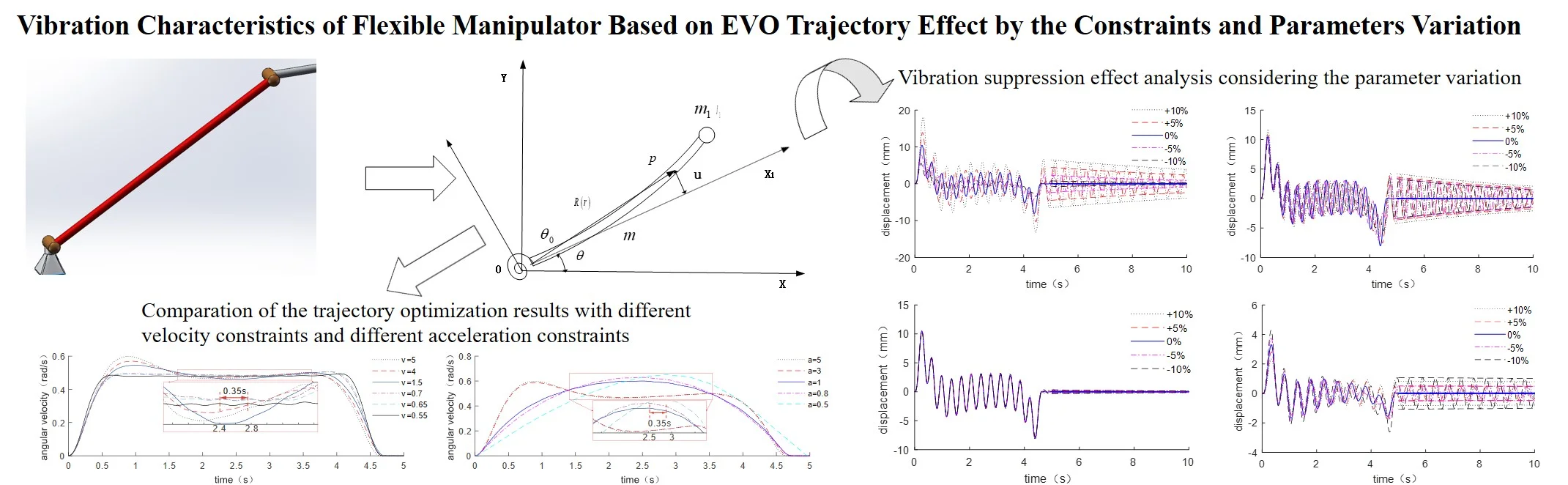
This paper studies the vibration control effect for manipulators with both flexible link and flexible joint according to the energy-vibration-optimal (EVO) trajectory planning method effect by the constraint conditions and structure parameters. First, a dynamic model of the flexible joint-flexible link arm is established following the assumed modal method and Lagrange principle. The optimization model is then proposed and discretized using the Particle Swarm Optimization (PSO) trajectory planning method and the trajectory optimization of discrete result algorithm, taking into account both residual oscillation and energy consumption. Following that, the numerical trajectory optimization results and their vibration suppression effect analysis by different constraint conditions, such as driving constraints, time constraints, and joint stiffness, are compared and discussed. The results show that the optimization velocity trajectory tends to a S-shaped trajectory and a convex trajectory respectively with the increase of driving velocity constraint and acceleration constraint respectively, while the sufficient planning time can make the less energy consumption. The parameter variations of length, cross-sectional area and next link lumped mass of have a significant impact on the residual oscillation of the flexible arm, with length having the most influence, whereas joint stiffness has little influence on the residual oscillation of the flexible link. The processing accuracy of length, cross-sectional area and end quality parameters must be ensured, while joint stiffness accuracy requirements can be slightly relaxed during the actual processing. Finally, experiments show that the optimization method is effective at vibration suppression. While the small variations of the end mass have significant influence on the vibration suppression effect, the residual vibrations of the parameter variation ones are all larger than the original parameter one. Meanwhile, as the mass of the manipulator increases, so does its energy consumption.
Highlights
- This paper studies the vibration reduction for manipulators with both flexible link and flexible joint according to the energy-vibration-optimal (EVO) trajectory planning method effect
- This paper studies the effect of changing the constraint value on the optimized trajectory in the PSO algorithm
- The impact of time constraints, joint stiffness constraints, and parameter changes on trajectory optimization and vibration suppression are discussed in order to enhance the efficiency and practicability of this method in practical applications
1. Introduction
Compared with traditional rigid manipulators, the flexible manipulator has gradually become a hot spot in robotics research due to its light weight, good flexibility, and low energy consumption owing to the rapid development of space manipulator technology in the aerospace field. The space flexible manipulator can help astronauts in space station with their daily maintenance work, high-precision and repetitive work, as well as high-risk extravehicular experiments, and so on, thereby enhancing astronaut safety and work efficiency. However, due to the influence of joint flexibility and link flexibility, the manipulator cannot reach the expected position and complete the expected work during the movement process as quickly and accurately as rigid manipulators, prompting researchers to pay increasing attention to mechanical arm vibration control.
The flexible manipulator is a strongly coupled nonlinear system. The establishment of accurate and applicable mathematical models is crucial for the study of its dynamics. The Newton-Euler method, the Lagrange method, and the Kane method are commonly used in the dynamic modeling of flexible links. Bascetta established the closed-form dynamic model of the flexible manipulator based on the Newton-Euler method [1] and the dynamic model of the highly flexible three-dimensional manipulator [2]. Esfandiar [3] and Martins [4]used Lagrange method and assumed mode method to model the dynamics of a single degree of freedom flexible rod. Buffinton [5, 6] used Kane's method to study the motion equations of a beam that moves longitudinally at a specified rate on both sides of the beam and a flexible robot that includes a moving pair. The complexity of the flexible manipulator system is reflected not only in the dynamic modeling method, but also has great difficulties in vibration control. Vibration reduction methods are broadly classified into two types: active control and passive control. For the active control of a flexible manipulator, Tzes [7] designed the application of an input precompensation scheme for vibration suppression in slewing flexible structures, with particular application to flexible-link robotic manipulator systems. Payo [8] proposed a feedback The control law, through the feedback loop control of the coupling torque between the motor and the flexible link, realizes the tracking of the contact force exerted by the flexible manipulator link in contact with a stationary object. Sarkhel [9] used a traditional PID controller to achieve precise control of the tip position of the flexible manipulator, and adjusts its gain value in different ways. Zaare [10] proposed a voltage-based sliding mode control (SMC) to control the position of n rigid-link flexible-joint (RLFJ) serial robot manipulator in the presence of structured and unstructured uncertainties. The passive control method uses damping materials to accelerate the attenuation of residual vibration. For example, Lew [11] took a single-link flexible manipulator as an example to illustrate the influence of passive damping on the position of the pole and zero of the system. Belherazem [12] studied the adaptive passive control of a single-link flexible manipulator with parameter uncertainties. In addition to passive control, many advances have been made in energy saving and vibration reduction trajectory planning in recent years. Considering the existing energy-saving trajectory generation algorithm is complicated and difficult to be used in real-time industrial control, CHEN [13] proposed an energy-saving fast generation algorithm for trapezoidal trajectory which is widely used in industrial practice. Li [14] proposed a method be used for on-line planning of vibration suppression trajectory in the process of manipulator motion. Zhang [15] Han [16] and Wang [17] presented a new trajectory planning methodology for manipulators respectively. Serrantola [18] and Khan [19] proposed a new algorithm to plan the manipulator's trajectory, respectively. Qiu [20] proposed a non-contact vibration measurement method based on structural light sensor. Jamali [21] established a controller algorithm for trajectory planning control and vibration cancelation of flexible manipulators. Although there are numerous active control algorithms for controlling the end vibration of the manipulator, the effectiveness of these methods is dependent on the placement and accuracy of the sensors. Whereas in some extreme environments, it is not appropriate to install sensors. Therefore, the active control based on trajectory planning without additional sensors remains an important research topic. In comparison to the commonly used trapezoidal trajectory control, polynomial S-shaped trajectory control, and other control methods, PSO is a stochastic search method yet with simpler philosophy. It was inspired by the coordinated motion of swarmed animals like flying birds and swimming fishes [22]. For example, Li [14] used residual energy of vibration as an objective function, the optimizer based on Particle Swarm Optimization (PSO) intelligent search algorithm is employed to search the motion trajectory of the manipulator with the best vibration suppression effect. Han [23] proposed a particle swarm optimization (PSO) algorithm which can dynamically adjust learning factors to solve the problems of low efficiency and unstable operation of traditional industrial robots. Wang [24] introduced a new method for trajectory planning issue of kinematically redundant manipulator while cope with joint range, velocity, acceleration limits with different objectives. And PSO with adaptive inertia weight and various fitness functions and constraints is implemented to find the optimal solution for trajectory planning of free-floating space robot. However, the preceding article only discusses the problem of the maximum value of the speed and acceleration constraint boundary or the relationship between the constraint boundary and time in the PSO algorithm, and does not discuss the effect of changing the constraint value on the optimized trajectory. Then, while Cui’s [25] paper discussed the impact of two distinct starting positions and limitations on vibration suppression, it did not consider the impact of changes in constraints on the optimized trajectory separately. Therefore, the results of trajectory optimization under various driving constraints are compared and discussed in this paper. Simultaneously, the impact of time constraints, joint stiffness constraints, and parameter changes on trajectory optimization and vibration suppression are discussed in order to enhance the efficiency and practicability of this method in practical applications.
In this paper, the trajectory optimization results with constraints and the vibration suppression effect of a manipulator with both joint flexibility and link flexibility are considered. Whereas the link is equivalent to Euler beam and the Assumption Modal Method is used to describe the elastic deformation of the link, and the flexible joint was simplified into a linear torsion spring model using Spong’s theory. The flexible joint-flexible link dynamic model was run using the Lagrange equation. The energy-vibration optimal method is used to propose a flexible trajectory optimization model in which the objective function and constraints are discretized, and the original complex constraint problem is discretized into a simple planning problem. Furthermore, the trajectory optimization results and vibration characteristics of the flexible arm are discussed in relation to the trajectory planning result based on PSO algorithm, where the vibration suppression effects considering the parameter variation are numerically compared simulated, and its vibration suppression effect is analyzed. Finally, an experiment platform with a flexible link is built, and the vibration control effect is validated.
2. Dynamic model of the flexible manipulator considering the joint flexibility and link flexibility
The flexible link of multi-link manipulator is shown in Fig. 1(a), where the subsequent links are considered as rigid part and assumed in static state. While its dynamic model is shown in Fig. 1(b), where the flexible joint is considered and the subsequent links are attached on the end of the flexible link. Where, the effect of the flexibility of the drive joint is equivalent to a linear spring with stiffness , and its rotation angle is ; is the drive joint’s moment of inertia; the flexible link is considered as uniform rod with Young’s modulus of elasticity , outer diameter , inner diameter , cross-sectional area A and cross-sectional moment of inertia , and , , are the length, mass and density of the flexible link respectively; is the rotation angle of the link, and u is the displacement; and are the lumped mass and inertia moment of next links; is the inertial coordinate system, while is rotating coordinate system bound to the flexible link.
Fig. 1Dynamic model of the flexible link in the multi-link manipulator
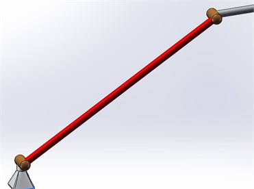
a) Flexible link of multi-link manipulator
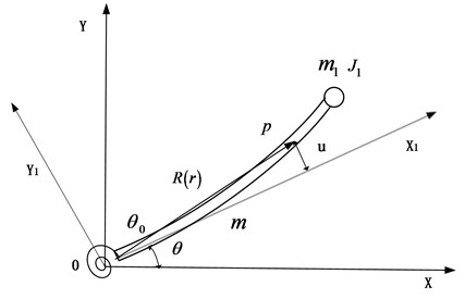
b) Dynamic model of the flexible link
The position of the point on the link in the rotating coordinate system and the inertial coordinate system can be expressed as and respectively:
The assumed mode method is used to discretize the flexible link by using the first two modes of the cantilever beam, and the elastic deformation and mode function of the flexible rod are:
where:
where, is the solution of the frequency equation . In this paper, the first two characteristic roots are taken, which can be written as , .
The system’s generalized coordinates are made up of the joint rotation angle, the flexible link rotation angle, the first-order modal coordinates and the second-order modal coordinates, which can be written as .
The overall kinetic energy of the link can be expressed as:
where, , , and are the rotational kinetic energy of the concentrated inertia at the drive, the kinetic energy of the flexible link and the kinetic energy of the lumped mass respectively, which can be expressed as:
The total potential energy of the link can be expressed as:
where, and are the elastic potential energy of the flexible link and the joint respectively, which can be expressed as:
The total energy dissipation of the system can be expressed as:
where, and are the dissipation energy generated by the damping of the flexible rod structure and the joint structure respectively, which can be expressed as:
where, is Rayleigh damping; is the joint damping coefficient. can be expressed as , where, and are the proportional coefficients, which can be expressed as , , and is the vibration frequency, which can be expressed as , and are the damping coefficient of the first-order mode and the second-order mode.
According to Lagrange equation:
The dynamic equations of the system can be expressed in matrix form as:
where, ; is the linear mass matrix; is the nonlinear mass matrix; is the linear damping matrix; is the nonlinear damping matrix; is the stiffness matrix; is the generalized force, which are shown as:
Suppose the link is rotated with small deformation, and use the Taylor expansion of the nonlinear term in Eq. (5) while ignoring high-order terms. Which is shown as:
Eq. (5) can be written as:
so:
where:
Defining:
in the Eq. (7) can be expressed as:
Eq. (7) can be written as:
Then the state equation can be written as:
where, . can be expressed as:
where .
3. Trajectory optimization model of flexible manipulator according to the energy-vibration optimal method
The trajectory optimization model is created using an energy-vibration optimum approach in this section. The system's energy consumption can be roughly calculated as the total of the energy spent during the motion process and the residual energy remaining after the motion. The amount of energy consumed during motion is proportional to the square of the motor output force [26], which may be approximated as:
The residual energy after the motion can be expressed as:
The optimum objective function can be converted from multi-objective planning to single-objective planning using the energy-vibration optimal approach:
which should satisfy constraint condition that , then there is:
Limited by the maximum velocity and acceleration of the motor, there are:
Eqs. (12)-(14) are the trajectory optimization model. In order to get the optimal trajectory, the objective function and constraints need to be discretized. Set the discretized time series as , if , the defined coordinate variable time series is , and the control variable time series is , then there is:
where, , . Eq. (10) can be discretized as:
where, , .
The diagonal matrix is defined as follows , where:
Then each discretized coordinate variable can be expressed as:
Eq. (12) can be discretized as:
where, , .
According to Eq. (13), Eq. (15) can be expressed as:
that is:
where, , .
Eq. (14) can express as:
where:
that is, , where:
Therefore, Eqs. (12)-(14) can be discretized into the following planning problem:
Only the mechanical work performed by the flexible link is taken into account when calculating the energy consumption during its movement. As a result, following discretization, the mechanical labor used during the entire movement is:
4. Trajectory optimization results analysis with different constraints
4.1. The influence of velocity and acceleration constraints on the optimized trajectory results
Table 1 shows the parameters of the simplified manipulator model depicted in Fig. 1.
Table 1Main parameters of the flexible dynamic model
Parameter | Unit | Value |
Length | m | 1.5 |
Density | kg/m3 | 2710 |
Outer diameter | m | 0.028 |
Inner diameter | m | 0.022 |
Young’s modulus | N/m2 | 7.1e10 |
Poisson’s ratio | – | 0.3 |
Drive joint stiffness | Nm/rad | 5e3 |
Drive joint damping | Nm/rad | 1.3e2 |
Inertia moment of drive joint | kg·m2 | 0.9e-3 |
In order to analyze the influence of the velocity and acceleration constraints on the optimized trajectory of the manipulator, different velocity and acceleration constraints are compared separately.
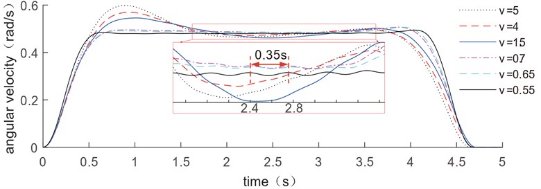
When only the drive velocity constraints works and the upper velocity constraints are 5 rad/s, 4 rad/s, 1.5 rad/s, 0.7 rad/s, 0.65 rad/s, and 0.55 rad/s separately, the optimized velocity trajectory results are shown in Fig. 2. When the upper velocity constraint is high, the optimized drive velocity curve shows a rapid increase in the early stage, and a slow decrease next. Then it gradually approaches a smooth movement with a fixed period, before gently approaching zero. With the decrease of the upper velocity constraint, the velocity trajectory gradually tends to a S-shape trajectory. The optimal trajectory is found to be close to an S-shaped trajectory only when the upper velocity constraint is less than 1.5 rad/s. The vibration period of the rod in Fig. 2 is 0.35 s, which is close to the first-order natural frequency of the flexible link 2.8329 Hz calculated by Eq. (4). The vibration frequency of the simulated physical model is found to be consistent with the theoretical calculation result.
Fig. 2Comparation of the trajectory optimization results with different velocity constraints
When only the drive acceleration constraints works and upper acceleration constraints are 5 rad/s2, 4 rad/s2, 1 rad/s2, 0.8 rad/s2, and 0.5 rad/s2 separately, the optimized velocity trajectory results are shown in Fig. 3. With the increase of the acceleration limit, the velocity trajectory gradually tends to a convex trajectory.
Fig. 3Comparation of the trajectory optimization results with different acceleration constraints
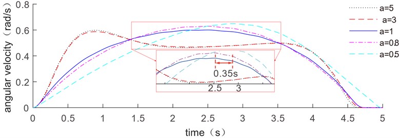
Fig. 4The optimized trajectory at vmax=5 rad/s, α= 5 rad/s2, α˙= 10 rad/s3
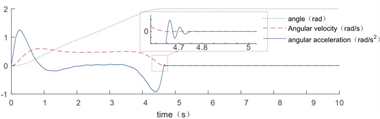
The optimized trajectory results of displacement, velocity, and acceleration are given in Fig. 4 where the upper velocity, upper acceleration, and upper jerk constraints are 5 rad/s, 5 rad/s2, and 10 rad/s3 respectively, and the trajectory optimization duration is from 0 s to 5 s.
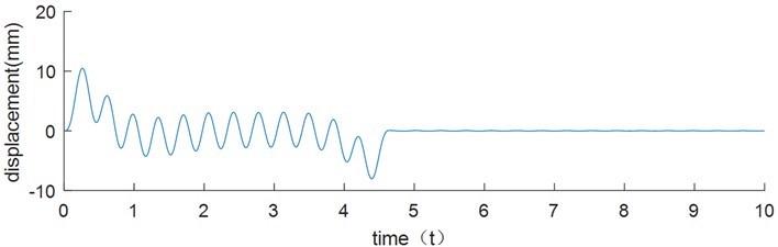
In order to observe vibration suppression effect of the optimized trajectories, the displacement vibration is shown in Fig. 5. Due to the nonlinear term is omitted during trajectory optimizing in Eqs. (5) and (6), the terminal vibration value is not zero when the driving motor stops. However, it can be found that the amplitude of the residual vibration is only 0.047 mm, which is close to zero. It has been demonstrated that this omission has no influence on vibration control, and that this optimization strategy has a significant effect on restraining the flexible link's vibration.
Fig. 5The end vibration of flexible link follows the optimized trajectory result
In order to show the vibration suppression effect of this method, we compare with different optimized trajectory methods and different control methods. Tao [27] proposed a novel trajectory planning scheme based on quintic polynomial transition to solve the conflict between swiftness and overshoot in traditional path planning as well as to suppress the vibration of flexible appendages. Hizarci [28] presents the development of an optimal PID controller by using PSO algorithm for position control of a flexible manipulator to reduce the vibration of the manipulator. In order to be more precise, the data from Berkan's paper is used for vibration suppression comparison. The flexible manipulator is made of stainless steel, having 0.414 m length, 0.026 m width, 0.0055 m thickness, 190 N/m2 elasticity modules, 7600 kg/m3 density and 13.4 g tip mass, 1 s planning time. The damping ratio estimated as 0.0038 under free vibration test [29].
Fig. 6The end vibration of flexible link follows the optimized trajectory result
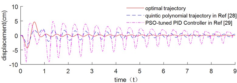
It can be seen from Fig. 6 that the optimal trajectory planning method has obvious vibration suppression effect compared with the quintic polynomial trajectory planning method and PSO tuned PID controller method. The end residual vibration of flexible link using three different approaches are illustrated in Table 2. Due to the nonlinear term is neglected during trajectory optimization in Eqs. (5) and (6), when moving at high speeds, the terminal vibration value when the drive motor stops is not zero. However, we can see that the optimal trajectory planning has a residual vibration of 0.46, which is below 2.06 and 2.81. As a result, the proposed trajectory planning scheme is significantly superior to the other two methods.
Table 2End residual vibration after t= 2 s
Different methods | End residual vibration (cm) |
Optimal trajectory | 0.46 |
Quintic polynomial trajectory [28] | 2.06 |
PSO-tuned PID Controller [29] | 2.81 |
4.2. The influence of time constraint on the optimized trajectory results
The influence of planning time on the optimal manipulator trajectory is analyzed and shown in Fig. 7 when the planning period is extended by 1 s and 2 s. The optimized trajectories of displacement, velocity, and acceleration have all been extended by the same amount of time, while the shape of the planning curves has remained relatively unchanged. Fig. 8 shows the end vibration and energy consumption of flexible link.
Fig. 7Comparation of the trajectory optimization results with different planning time
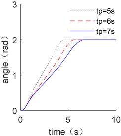
a) Displacement comparison
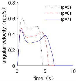
b) Velocity comparison
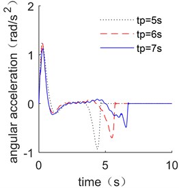
c) Acceleration comparison
Fig. 8End vibration and energy consumption of flexible link
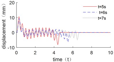
a) Comparison of end displacement
b) Comparison of energy consumption
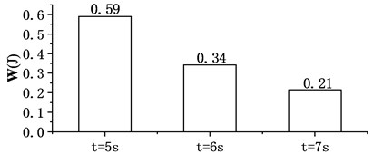
Figure 8(a) shows that all of the three optimization results have significant effect on restraining the vibration of the flexible link, with the maximum vibration decreasing as the of time constraint increases. Fig. 8(b) shows the results of energy consumption of driving motor. The overall energy consumption decreases as the planning time increases. It can be found that sufficient planning time can make the less vibration, which is more beneficial to suppress vibration.
4.3. The influence of joint stiffness on the optimized trajectory results
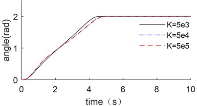
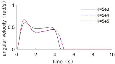
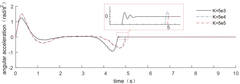
In order to analyze the influence of the joint stiffness on the optimized trajectory of the manipulator, results with 5000 Nm/rad, 50000 Nm/rad, 500000 Nm/rad are compared. Which is shown in Fig. 9.
As shown in Fig. 9, the raised edge of driving trajectory of displacement, velocity and acceleration are all shift to the right with the joint stiffness increases. It shows in Fig. 9(c) that the acceleration will converge to the values near zero in advance when the joint stiffness is very small; while when the stiffness is larger, it will converge to zero later or even close to 5 seconds. It also shows that the joint stiffness has a minor impact on the ideal trajectory.
Fig. 9Comparation of the trajectory optimization results with different joint stiffness
a) Displacement comparison
b) Velocity comparison
c) Acceleration comparison
5. Vibration suppression effect analysis considering the parameter variation
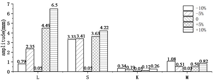
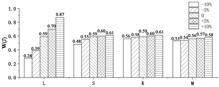
Parameter variation always has a significant influence on trajectory optimization. For the flexible manipulator, the length and cross-sectional area of the link, torsional stiffness of the joint, and the lumped mass of the next link are all important parameters for the driving trajectory optimization analysis. Therefore, the four different parameters including length , cross-sectional area , joint torsional stiffness and the lumped mass are considered and compared with different variations ranging from –10 % to 10 %. The dynamic responses follow the optimized trajectory results are shown in Fig. 10, while the residual vibrations and energy consumptions of the flexible manipulator are shown in Fig. 11.
Fig. 10(a), (b) and (d) show that the small variations in length, cross-sectional area, and lumped mass have a significant influence on the vibration suppression effect when compared to joint stiffness. The residual vibrations of the parameter variation ones are far larger than the original parameter one, as shown in Fig. 11(a). The energy consumption of manipulator increases as the length, cross-sectional area, joint stiffness and lumped mass increase, as shown in Fig. 11(b). The most significant impact on energy consumption is length variation, while joint stiffness has a minor influence. The processing accuracy of length, cross-sectional area and end quality parameters must be ensured in order to ensure the vibration suppression effect following the trajectory optimization result during actual processing. The change in torsional stiffness, on the other hand, has a minor impact on residual vibration and energy consumption, so joint stiffness accuracy criteria can be slightly relaxed.
Fig. 10The influence of parameter variation
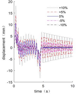
a) End displacement with different
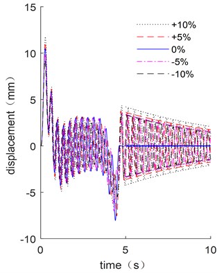
b) End displacement with different
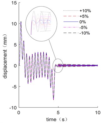
c) End displacement with different
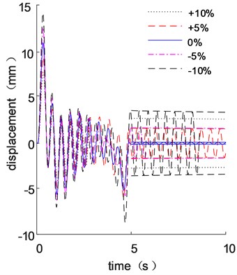
d) End displacement with different
6. Experiment and analysis
Fig. 12 shows a flexible manipulator test rig that is powered by a DC motor and has its velocities reduced by a 1:15 reducer to allow the flexible arm to move smoothly in accordance with the specified driving mode. The piezoelectric acceleration sensor attached to the end of the link collects vibration data from the flexible link, and the closed loop Hall sensor collects current variation during movement. As a result, according to , the energy consumption is calculated.
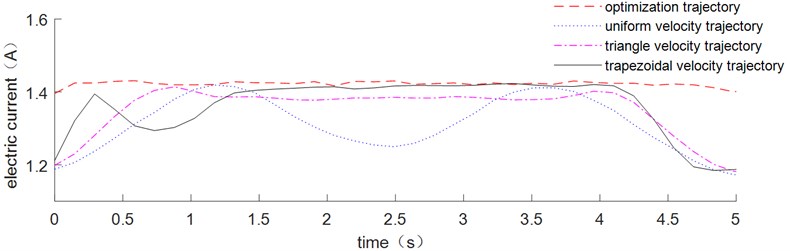
As shown in Fig. 13, four driving trajectories are compared: uniform velocity trajectory, triangle velocity trajectory, trapezoidal velocity trajectory and the optimal trajectory.
The corresponding acceleration signals at the end of the flexible link are shown in Fig. 14. When the motor starts or stops, it has a significant vibration impact. The optimal trajectory in Fig. 13 has the smallest residual vibration after the movement, while the uniform velocity trajectory has the greatest residual vibration.
The variation of driving currents after moving average are shown in Fig. 15, while the energy consumptions are shown in Table 3. The current curve and energy consumption of the link driven by the optimized trajectory are not the smallest, but their residual vibration is. Because the nonlinear term in Eqs. (5) and (6) is omitted during trajectory optimizing optimization, the residual vibration is zero, which is used as the prior constraint condition. However, it can be shown in Table 3 that the energy consumption of the four driving trajectories is not significantly different, whereas the residual vibration of the optimized trajectories is significantly lower than that of the other trajectories, proving that the optimized trajectory has a good vibration suppression effect.
Table 3Energy consumption of the end of the link
Driving trajectories | Energy consumption (J) |
Uniform velocity trajectory | 169.92 |
Triangle velocity trajectory | 157.53 |
Trapezoidal velocity trajectory | 162.21 |
Optimal trajectory | 163.50 |
Fig. 11residual vibrations and energy consumptions of the flexible manipulator with the parameter variation
a) Maximum end vibration after 5 s
b) Energy consumption
Fig. 12Flexible manipulator test rig
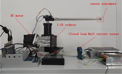
Fig. 13Four driving trajectories
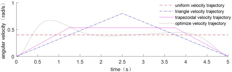
Fig. 14Acceleration of the end of the link
a) Uniform velocity trajectory
b) Triangle velocity trajectory
c) Trapezoidal velocity trajectory
d) Optimal trajectory
Fig. 15Current value with time
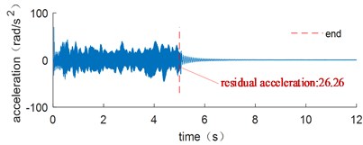
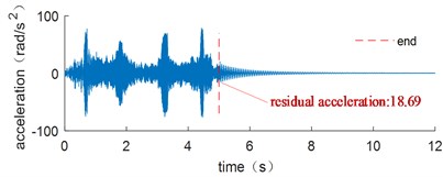
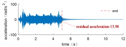
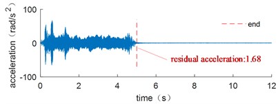
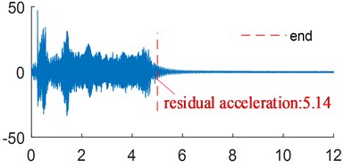
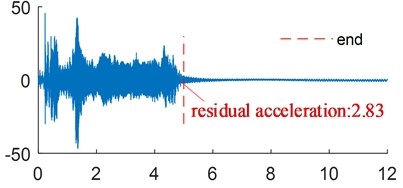
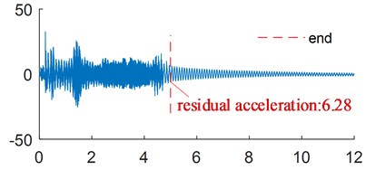
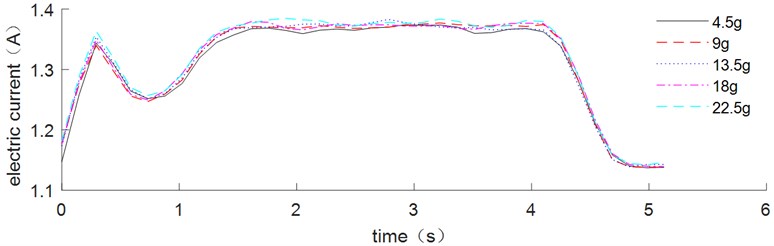
The vibration suppression effect of the flexible arm with 13.5 g end mass was analyzed. The corresponding acceleration signals are measured at the ends of flexible links with end masses of 4.5 g, 9 g, 13.5 g, 18 g and 22.5 g. The residual acceleration of the corresponding acceleration signals at the end of flexible link is shown in Fig. 16. The variation of current after moving average is shown in Fig. 17. Table 4 shows the residual acceleration and energy consumption of the end of the link.
As shown in Fig. 16, small variations in mass have a significant influence on the vibration suppression effect, and the residual vibrations of the parameter variation ones are all larger than the original parameter one. Table 4 shows that the energy consumption of the manipulator increases as the mass increase, which proves the previous simulation results.
Table 4Residual acceleration and energy consumption of the end of the link with different end mass
End mass (g) | Energy consumption (J) |
4.5 | 157.12 |
9 | 157.60 |
13.5 | 157.72 |
18 | 157.94 |
22.5 | 158.49 |
Fig. 16Acceleration of the end of the link with different end mass
a) 4.5 g end mass

b) 9 g end mass
c) 13.5 g end mass

d) 18 g end mass
e) 22.5 g end mass
Fig. 17Current value with time
7. Conclusions
The residual vibration and energy consumption of a manipulator with both flexible link and flexible joint that has a certain structure size is used as the objective function for trajectory planning and design using PSO trajectory planning method. In comparison to quadratic programming, the PSO has better stability and is more convenient for dealing with the optimization design problem of manipulators with both flexible link and flexible joint. The results of the trajectory optimization with different constraints, as well as vibration suppression effect analysis with parameter variation of the dynamic model driven by this optimized trajectory, are studied.
In order to analyze the influence of the velocity and acceleration constraints on the optimized trajectory of the manipulator, different velocity and acceleration constraints are compared separately. The velocity trajectory gradually tends to an S-shape trajectory as the upper velocity constraint is reduced. It has been found that the optimal trajectory will close to an S-shaped trajectory only when the upper velocity constraint is less than a certain value. And as the acceleration limit is increased, the velocity trajectory gradually tends to a convex trajectory. Meanwhile, adequate planning time can reduce vibration, which is more beneficial to vibration suppression, whereas joint stiffness has a minor influence on the optimal trajectory result. It was discovered that the constraint effect has a significant effect on the shape of optimal trajectory.
Small variations in length, cross-sectional area, and lumped mass have a significant influence on the vibration suppression effect when compared to joint stiffness; the residual vibrations of the parameter variation ones are far larger than the original parameter one. The energy consumption of the manipulator increases as the length, cross-sectional area, joint stiffness, and the end mass increase. The length variation has the greatest impact on energy consumption, while joint stiffness has a minor impact. To ensure the vibration suppression effect following the trajectory optimization result during actual processing, the processing accuracy of length, cross-sectional area and end quality parameters must be ensured. Whereas the change in residual vibration and energy consumption caused by torsional stiffness is relatively small. The accuracy requirements for joint stiffness can be slightly relaxed.
The experiment is conducted using flexible manipulator test rig. It demonstrates that the optimal trajectory has a good suppression effect on the flexible manipulator. The residual vibrations of the parameter variation ones are larger than the original parameter one, and the energy consumption of the manipulator increases as the end mass increases. it proves that small variations in lumped mass have a significant impact on the vibration suppression.
References
-
L. Bascetta, G. Ferretti, and B. Scaglioni, “Closed form Newton-Euler dynamic model of flexible manipulators,” Robotica, Vol. 35, No. 5, pp. 1006–1030, May 2017, https://doi.org/10.1017/s0263574715000934
-
B. Scaglioni, L. Bascetta, M. Baur, and G. Ferretti, “Closed-form control oriented model of highly flexible manipulators,” Applied Mathematical Modelling, Vol. 52, pp. 174–185, Dec. 2017, https://doi.org/10.1016/j.apm.2017.07.034
-
H. Esfandiar and S. Daneshmand, “Complete dynamic modeling and approximate state space equations of the flexible link manipulator,” Journal of Mechanical Science and Technology, Vol. 26, No. 9, pp. 2845–2856, Sep. 2012, https://doi.org/10.1007/s12206-012-0731-x
-
J. Martins, M. Ayala Botto, and J. Sá Da Costa, “Modeling of flexible beams for robotic manipulators.,” Multibody System Dynamics, Vol. 7, No. 1, pp. 79–100, 2002, https://doi.org/10.1023/a:1015239604152
-
K. W. Buffinton and T. R. Kane, “Dynamics of a beam moving over supports,” International Journal of Solids and Structures, Vol. 21, No. 7, pp. 617–643, 1985, https://doi.org/10.1016/0020-7683(85)90069-1
-
K. W. Buffinton, “Dynamics of elastic manipulators with prismatic joints,” Journal of Dynamic Systems, Measurement, and Control, Vol. 114, No. 1, pp. 41–49, Mar. 1992, https://doi.org/10.1115/1.2896506
-
A. Tzes and S. Yurkovich, “An adaptive input shaping control scheme for vibration suppression in slewing flexible structures,” IEEE Transactions on Control Systems Technology, Vol. 1, No. 2, pp. 114–121, Jun. 1993, https://doi.org/10.1109/87.238404
-
I. Payo, V. Feliu, and O. D. Cortázar, “Force control of a very lightweight single-link flexible arm based on coupling torque feedback,” Mechatronics, Vol. 19, No. 3, pp. 334–347, Apr. 2009, https://doi.org/10.1016/j.mechatronics.2008.10.003
-
P. Sarkhel, N. Banerjee, and N. B. Hui, “Fuzzy logic-based tuning of PID controller to control flexible manipulators,” SN Applied Sciences, Vol. 2, No. 6, p. 1124, Jun. 2020, https://doi.org/10.1007/s42452-020-2877-y
-
S. Zaare, M. R. Soltanpour, and M. Moattari, “Voltage based sliding mode control of flexible joint robot manipulators in presence of uncertainties,” Robotics and Autonomous Systems, Vol. 118, pp. 204–219, Aug. 2019, https://doi.org/10.1016/j.robot.2019.05.014
-
J. Y. Lew and M. S. Evans, “The effect of passive damping on feedback control performance of flexible manipulators,” in American Control Conference, Jun. 1994.
-
A. Belherazem and M. Chenafa, “Passivity based adaptive control of a single-link flexible manipulator,” Automatic Control and Computer Sciences, Vol. 55, No. 1, pp. 1–14, Jan. 2021, https://doi.org/10.3103/s0146411621010028
-
H. Chen, “Real-time generation of trapezoidal velocity profile for energy saving in servomotor systems,” Journal of Mechanical Engineering, Vol. 54, No. 7, p. 152, 2018, https://doi.org/10.3901/jme.2018.07.152
-
Y. Li, S. S. Ge, Q. Wei, T. Gan, and X. Tao, “An online trajectory planning method of a flexible-link manipulator aiming at vibration suppression,” IEEE Access, Vol. 8, pp. 130616–130632, 2020, https://doi.org/10.1109/access.2020.3009526
-
S. Zhang, S. Dai, A. M. Zanchettin, and R. Villa, “Trajectory planning based on non-convex global optimization for serial manipulators,” Applied Mathematical Modelling, Vol. 84, pp. 89–105, Aug. 2020, https://doi.org/10.1016/j.apm.2020.03.004
-
Y. Han, K. Zhao, Z. Chu, and Y. Zhou, “Grasping control method of manipulator based on binocular vision combining target detection and trajectory planning,” IEEE Access, Vol. 7, pp. 167973–167981, 2019, https://doi.org/10.1109/access.2019.2954339
-
Q. Wang, Z. Wang, and M. Shuai, “Trajectory planning for a 6-DoF manipulator used for orthopaedic surgery,” International Journal of Intelligent Robotics and Applications, Vol. 4, No. 1, pp. 82–94, Mar. 2020, https://doi.org/10.1007/s41315-020-00117-4
-
W. G. Serrantola and V. Grassi, “Trajectory planning for a dual-arm planar free-floating manipulator using RRT control,” in 2019 19th International Conference on Advanced Robotics (ICAR), pp. 394–399, Dec. 2019, https://doi.org/10.1109/icar46387.2019.8981596
-
A. T. Khan, S. Li, S. Kadry, and Y. Nam, “Control framework for trajectory planning of soft manipulator using optimized RRT algorithm,” IEEE Access, Vol. 8, pp. 171730–171743, 2020, https://doi.org/10.1109/access.2020.3024630
-
Z.-C. Qiu and W.-Z. Zhang, “Trajectory planning and diagonal recurrent neural network vibration control of a flexible manipulator using structural light sensor,” Mechanical Systems and Signal Processing, Vol. 132, pp. 563–594, Oct. 2019, https://doi.org/10.1016/j.ymssp.2019.07.014
-
A. Jamali and I. Z. Mat Darus, “Intelligent evolutionary controller for flexible robotic arm,” in Journal of Physics: Conference Series, Vol. 1500, No. 1, p. 012020, Apr. 2020, https://doi.org/10.1088/1742-6596/1500/1/012020
-
R. Eberhart and J. Kennedy, “A new optimizer using particle swarm theory,” in MHS’95. Proceedings of the Sixth International Symposium on Micro Machine and Human Science, pp. 39–43, 1995, https://doi.org/10.1109/mhs.1995.494215
-
S. Han, X. Shan, J. Fu, W. Xu, and H. Mi, “Industrial robot trajectory planning based on improved PSO algorithm,” in Journal of Physics: Conference Series, Vol. 1820, No. 1, p. 012185, Mar. 2021, https://doi.org/10.1088/1742-6596/1820/1/012185
-
M. Wang, J. Luo, and U. Walter, “Trajectory planning of free-floating space robot using Particle Swarm Optimization (PSO),” Acta Astronautica, Vol. 112, pp. 77–88, Jul. 2015, https://doi.org/10.1016/j.actaastro.2015.03.008
-
L. Cui, H. Wang, and W. Chen, “Trajectory planning of a spatial flexible manipulator for vibration suppression,” Robotics and Autonomous Systems, Vol. 123, No. 6, p. 103316, Jan. 2020, https://doi.org/10.1016/j.robot.2019.103316
-
K.-S. Low and T.-S. Wong, “A multiobjective genetic algorithm for optimizing the performance of hard disk drive motion control system,” IEEE Transactions on Industrial Electronics, Vol. 54, No. 3, pp. 1716–1725, Jun. 2007, https://doi.org/10.1109/tie.2007.894709
-
J. Tao, T. Zhang, Y. Wang, and S. Tan, “Attitude control and vibration suppression of flexible spacecraft based on quintic polynomial path planning,” in 2017 29th Chinese Control and Decision Conference (CCDC), May 2017, https://doi.org/10.1109/ccdc.2017.7978713
-
H. Hizarci and S. Ikizoglu, “Position control of flexible manipulator using PSO-tuned PID controller,” in 2019 Innovations in Intelligent Systems and Applications Conference (ASYU), Oct. 2019, https://doi.org/10.1109/asyu48272.2019.8946440
About this article

The study was supported by the Natural Science Foundation of Liaoning Province (granted No. 2019-KF-01-08) and Key Laboratory of Vibration and Control of Aero-Propulsion System Ministry of Education, Northeastern University (granted No. VCAME201903).
