On the use of Maggi’s equation in the dynamic modeling of multibody systems

Horn, Arthur; Malvezzi, Fernando; Orsino, Renato M. M.

doi:10.21595/vp.2020.21323

Vibroengineering Procedia

Browse Procedia

Published: 29 June 2020

Check for updates

On the use of Maggi’s equation in the dynamic modeling of multibody systems

Arthur Horn¹

Fernando Malvezzi²

Renato M. M. Orsino³

¹Mechanical Engineering Department, Escola Politécnica, University of São Paulo, São Paulo, Brazil

^{2, 3}Mechanical Engineering Department, Mauá Institute of Technology, São Caetano do Sul, Brazil

Corresponding Author:

Arthur Horn

Cite the article Download PDF

Downloads 1164

CrossRef Citations 1

Abstract

The purpose of dynamic modeling of multibody mechanical systems is to obtain the differential equations of motion. Maggi’s equation appears as an alternative to obtain the differential equations of motion. The aim of this work is to illustrate the advantages of the use of Maggi's equation in the dynamic modeling of multibody mechanical systems. Maggi's equation is used to model the dynamics of a classical complex constrained mechanical system. An inverse dynamics simulation is performed, to illustrate how the obtained equations can be used to determine the theoretical time series of the torques required to perform a given prescribed trajectory.

On the use of Maggi’s equation in the dynamic modeling of multibody systems

Highlights

Maggi's equations were used to derive a complete non-linear dynamic model for a 6 degrees of freedom mechanism
The use of redundant generalized coordinates led to significant simplification in the terms related to kinetic and potential energy
The use of Baumgarte method avoided the presence of numerical instability which is associated with the violation of constraints equations during numerical integration
The approach employed to obtain the differential equations of motion might be useful for dynamic modeling of other multiple-degree-of-freedom multibody systems

1. Introduction

Maggi’s equations were introduced by Gian Antonio Maggi in 1896 as an alternative approach to deal with constrained multibody systems (with either holonomic or linear non-holonomic constraints). As described in [1], Maggi’s equation can be understood as an extension of Lagrangian formalism that, by means of a simple algorithm based on finding a linear operator onto the kernel of the constraint equations Jacobian, allows the elimination of the undetermined multipliers from the equations of motion of a constrained mechanical.

Whenever redundant generalized coordinates are used in a given formulation (which is inevitable in the case of non-holonomic systems and might be convenient for holonomic ones), the requirement of using indeterminate multipliers in the conventional Lagrangian formalism arises, leading to a system of differential-algebraic equations of motion (DAEs) instead of simply ordinary differential equations (ODEs) [2, 3].

Even though Maggi’s equation provides an alternative formalism in which the undetermined multipliers are eliminated, problems associated with the numerical integration of DAEs, due to violation of constraint equations are still present. Baumgarte method provides an stabilization algorithm in order to improve the numerical accuracy of the numerical solution of these equations [4].

Malvezzi et al. [5] and Orsino et al. [6] proposed a qualitative comparison based on the use of Lagrange’s, Maggi’s and Kane’s equations applied to the modelling of multibody mechanical systems. In those papers, it has been shown that the application of Maggi’s equations, combined with a proper choice of a redundant set of generalized coordinates, leads to a simpler derivation of the dynamic equations of motion, in a suitable form for numerical simulations. Moreover, it also has been shown that, the procedure for adding new bodies and obtaining differential equations of motion without the terms related to constraints forces is simple.

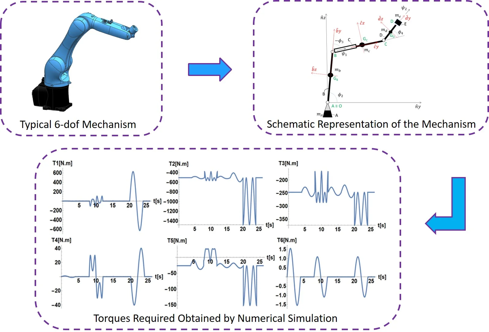
Newton-Euler equations and Lagrange equations are mostly used in the dynamic modeling of many-degree-of-freedom multibody systems. As an alternative to the above approach, the purpose of this paper is to illustrate the advantages of applying Maggi’s equations along with a solid formalism. The chosen system is a serial six degrees of freedom (6-dof) robot manipulator, a classical example of a complex constrained mechanical system. Finally, in order to investigate the numerical performance of the equations of motion obtained by this approach, an inverse dynamics simulation is performed, to obtain the theoretical time series of the torques required to perform a proposed trajectory.

2. Differential equation of motion

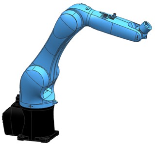
This section details the derivation of the differential equations of motion of the 6-dof serial mechanism illustrated in Fig. 1. This mechanism consists of 5 rigid bodies (A, B, C, D and E). It is noteworthy that the bodies C and E can perform rotations around the axes ${\hat{c}}_{y}$ and ${\hat{d}}_{y}$ , respectively, properly controlled by actuators.

2.1. Mechanical system

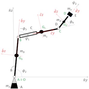
Fig. 1(a) illustrates the typical six degree of freedom mechanical system that was chosen to be studied, while Fig. 1(b) shows its schematic representation.

Fig. 1a) Typical mechanism, b) schematic representation of the 6-dof mechanism in a configuration in which the centerlines of the links remain in the Oyz plane

a) Typical mechanism, b) schematic representation of the 6-dof mechanism in a configuration in which the centerlines of the links remain in the Oyz plane

a)

b)

Fig. 1(b) shows a schematic representation of the mechanism illustrating the angular coordinates and coordinate systems adopted in the modeling. The rigid bodies and the coordinate system fixed to the bodies are represented by black capital letter and the points identifications are represented by green underlined capital letter.

Table 1Definition of generalized coordinates

Generalized coordinate	Definition
$γ$	Rotation angle around ${\hat{n}}_{z}$
$ϕ_{2}$	Angle between the direction ${\hat{b}}_{y}$ and the plane $O x y$
$ϕ_{3}$	Angle between the directions ${\hat{b}}_{y}$ and ${\hat{c}}_{y}$
$ψ_{1}$	Rotation angle around ${\hat{c}}_{y}$
$ϕ_{4}$	Angle between the directions ${\hat{c}}_{y}$ and ${\hat{d}}_{y}$
$ψ_{2}$	Rotation angle around ${\hat{d}}_{y}$

The following hypotheses are adopted in the derivation of the mathematical model: all the bodies are considered rigid bodies; all joints are ideal and the axes ${\hat{a}}_{x}$ , ${\hat{a}}_{y}$ , ${\hat{a}}_{z}$ , ${\hat{b}}_{x}$ , ${\hat{b}}_{y}$ , ${\hat{b}}_{z}$ , ${\hat{c}}_{x}$ , ${\hat{c}}_{y}$ , ${\hat{c}}_{z}$ , ${\hat{d}}_{x}$ , ${\hat{d}}_{y}$ and ${\hat{d}}_{z}$ correspond to the principal axes of inertia of the respective bodies.

2.2. Mathematical modeling

2.2.1. Notation

Regarding the kinematic description of the system, consider the following notation:

– $R_{I}^{H}$ is the rotation matrix between the bases of the coordinate systems H and I.

– $p_{G | O}^{F}$ is the column-matrix representation, with components expressed in the base of the coordinate system F, of the position vector of point G with respect to point O.

– $ω_{H | I}^{F}$ is the column-matrix representation, with components expressed in the base of the coordinate system F, of the angular velocity vector of body H with respect to the reference frame (or rigid-body) I.

2.2.2. Constraints

In order to use redundant generalized coordinates, a matrix of generalized coordinates is defined:

1

q^{T} = [γ ϕ_{2} ϕ_{3} ψ_{1} ϕ_{4} ψ_{2} x_{B} y_{B} z_{B} x_{C} y_{C} z_{C} x_{D} y_{D} z_{D} x_{E} y_{E} z_{E}] .

The generalized coordinates $x_{B}$ , $y_{B}$ , $z_{B}$ , $x_{C}$ , $y_{C}$ , $z_{C}$ , $x_{D}$ , $y_{D}$ , $z_{D}$ , $x_{E}$ , $y_{E}$ and $z_{E}$ are the Cartesian coordinates of the respective centers of mass of the bodies A, B, C, D and E in the coordinate system $N$ . Thus, a mechanical system of 6 degrees of freedom ( $v$ ), with 18 generalized coordinates ( $n$ ), requires 12 constraints equations to be defined ( $p$ ). In order to obtain the constraints equations, the following position vectors is defined:

2

p_{A | O}^{A} = {[0 0 0]}^{T}, p_{G_{B} | O}^{B} = {[0 η l_{1} 0]}^{T}, p_{B | O}^{B} = {[0 l_{1} 0]}^{T},

3

p_{G_{C} | B}^{C} = {[0 ν l_{2} 0]}^{T}, p_{C | B}^{C} = {[0 l_{2} 0]}^{T}, p_{G_{D} | C}^{D} = {[0 ϵ l_{3} 0]}^{T},

4

p_{D | C}^{D} = {[0 l_{3} 0]}^{T}, p_{G_{B} | O}^{N} = R_{A}^{N} . R_{B}^{A} . p_{G_{B} | O}^{B}, p_{B | O}^{N} = R_{A}^{N} . R_{B}^{A} . p_{B | O}^{B},

5

p_{G_{C} | O}^{N} = R_{A}^{N} {. R}_{B}^{A} . R_{C}^{B} . p_{G_{C} | B}^{C} + p_{B | O}^{N}, p_{C | O}^{N} = R_{A}^{N} . R_{B}^{A} . R_{C}^{B} . p_{C | B}^{C} + p_{B | O}^{N},

6

p_{G_{D} | O}^{N} = R_{A}^{N} . R_{B}^{A} . R_{C}^{B} R_{D}^{C} . p_{G_{D} | C}^{D} + p_{C | O}^{N}, p_{D | O}^{N} = R_{A}^{N} R_{B}^{A} . R_{C}^{B} . R_{D}^{C} . p_{D | C}^{D} + p_{C | O}^{N} .

Thus, it is possible to relate the Cartesian coordinates of the center of gravity of the bodies with the generalized angular coordinates. These constraint equations can be expressed in the form $h (t, q) = 0$ , whose time derivative can be expressed by the following Pfaff form Eq. (7) [1]:

7

\dot{h} (t, q, \dot{q}) = A_{*} (t, q) \dot{q} - b_{*} (t, q) = 0 .

Let $A_{#}$ be a matrix $v$ × $n$ , ( $v$ – number of degrees of freedom, $n$ – number of generalized coordinates) chosen to make the following matrix invertible [1]:

8

E = [\begin{matrix} A_{#} \\ A_{*} \end{matrix}], E^{- 1} = [\begin{matrix} S_{#} & S_{*} \end{matrix}] .

2.2.3. Stabilization of constraints

In order to improve the numerical stability of the constraint enforcement in the numerical simulations, the Baumgarte method [4] was used:

9

\ddot{h} + 2 ζ β \dot{h} + β^{2} h = 0 .

With 𝛽 and 𝜁 being empirically defined parameters.

2.2.4. Kinematics

Considering the angular coordinates defined in Table 1, the following expressions can be written for angular velocity vectors:

10

ω_{A | N}^{A} = {[0 0 \dot{γ}]}^{T}, ω_{B | A}^{B} = {[{\dot{ϕ}}_{2} 0 0]}^{T}, ω_{C | B}^{C} = {[{\dot{ϕ}}_{3} \dot{ψ_{1}} 0]}^{T}

11

ω_{D | C}^{D} = {[\dot{ϕ_{4}} 0 0]}^{T}, ω_{E | D}^{D} = {[0 \dot{ψ_{2}} 0]}^{T}, ω_{A | N}^{A} = {[0 0 \dot{γ}]}^{T}

12

ω_{B | N}^{B} = {R_{B}^{A}}^{- 1} . ω_{A | N}^{A} + ω_{B | A}^{B}, ω_{C | N}^{C} = {R_{C}^{B}}^{- 1} . ω_{B | N}^{B} + ω_{C | B}^{C}

13

ω_{D | N}^{D} = {R_{D}^{C}}^{- 1} . ω_{C | N}^{C} + ω_{D | C}^{D}, ω_{E | N}^{D} = ω_{D | N}^{D} + ω_{E | D}^{D} .

2.2.5. Kinetic energy

The expression for the kinetic energy of this mechanism can be expressed as follows:

14

T = \frac{1}{2} m_{B} ({\dot{x_{B}}}^{2} + {\dot{y_{B}}}^{2} + {\dot{z_{B}}}^{2}) + \frac{1}{2} m_{C} ({\dot{x_{C}}}^{2} + {\dot{y_{C}}}^{2} + {\dot{z_{C}}}^{2}) + \frac{1}{2} m_{D} ({\dot{x_{D}}}^{2} + {\dot{y_{D}}}^{2} + {\dot{z_{D}}}^{2}) + \frac{1}{2} m_{E} ({\dot{x_{E}}}^{2} + {\dot{y_{E}}}^{2} + {\dot{z_{E}}}^{2}) + \frac{1}{2} ({ω_{A | N}^{A}}^{T} . J_{A} . ω_{A | N}^{A}) + \frac{1}{2} ({ω_{B | N}^{B}}^{T} . J_{B} . ω_{B | N}^{B}) + \frac{1}{2} ({ω_{C | N}^{C}}^{T} . J_{C} . ω_{C | N}^{C}) + \frac{1}{2} ({ω_{D | N}^{D}}^{T} . J_{D} . ω_{D | N}^{D}) + \frac{1}{2} ({ω_{E | N}^{D}}^{T} . J_{E} . ω_{E | N}^{D}) .

Observing Eq. (14), it can be noticed that the use of redundant generalized coordinates significantly simplifies the description of the kinetic energy of the system, making the role of each term in this expression easier to interpret. The first four terms make up the parcel of the kinetic energy associated with the translational motion of bodies B, C, D and E, while the last five terms make up the parcel of the kinetic energy associated with the rotational motion of bodies A, B, C, D and E.

2.2.6. Potential energy

The potential energy of the mechanical system can be described as follows:

15

V = m_{B} g z_{b} + m_{c} g z_{c} + m_{d} g z_{d} + m_{e} g z_{e} .

2.2.7. Generalized forces

The generalized forces acting on the mechanical system are the torques exerted by the actuators located on the revolute joints. Thus, corresponding non-conservative generalized forces are:

16

Q_{γ} = T_{1}, Q_{ϕ_{2}} = T_{2}, Q_{ϕ_{3}} = T_{3}, Q_{ψ_{1}} = T_{4}, Q_{ϕ_{4}} = T_{5}, Q_{ψ_{2}} = T_{6} .

2.2.8. Differential equations of motion

Based on the previously defined expressions, and considering that $L = T - V$ is the Lagrangian of the system, the equations of motion for the 6-dof mechanism can be directly obtained for Maggi’s equations:

17

S_{#}^{T} . [\frac{d}{d t} \frac{\partial L}{\partial {\dot{q_{i}}}} - \frac{\partial L}{\partial {{q}_{i}}} - Q_{q_{i}}] = 0 .

3. Numerical simulations

Adopting the equations of motion derived in the last section, a numerical simulation scenario was proposed. In this section an inverse dynamics simulation is performed, in order to determine the theoretical time series of the torques required to perform a given prescribed trajectory. Table 2 shows the mechanism parameters adopted in the numerical simulation.

Table 2Mechanism parameters used in the numerical simulation

Mechanism Parameters	Value
Moment of inertia of the body A with respect to the ${\hat{a}}_{z}$ axis [kgm²]	3.0
Mass of body B [kg]	3.0
Length of body B [m]	1.0
Moment of inertia of the body B with respect to the ${\hat{b}}_{x}$ axis [kgm²]	0.4
Moment of inertia of the body B with respect to the ${\hat{b}}_{y}$ axis [kgm²]	0.1
Moment of inertia of the body B with respect to the ${\hat{b}}_{z}$ axis [kgm²]	0.4
Mass of body C [kg]	3.0
Length of body C [m]	1.0
Moment of inertia of the body C with respect to the ${\hat{c}}_{x}$ axis [kgm²]	0.4
Moment of inertia of the body C with respect to the ${\hat{c}}_{y}$ axis [kgm²]	0.1
Moment of inertia of the body C with respect to the ${\hat{c}}_{z}$ axis [kgm²]	0.4
Mass of body D [kg]	0.3
Length of body D [m]	3.0
Moment of inertia of the body D with respect to the ${\hat{d}}_{x}$ axis [kgm²]	0.2
Moment of inertia of the body D with respect to the ${\hat{d}}_{y}$ axis [kgm²]	0.05
Moment of inertia of the body D with respect to the ${\hat{d}}_{z}$ axis [kgm²]	0.2
Mass of body E [kg]	3.0
Moment of inertia of the body E with respect to the ${\hat{d}}_{x}$ axis [kgm²]	0.2
Moment of inertia of the body E with respect to the ${\hat{d}}_{y}$ axis [kgm²]	0.2
Moment of inertia of the body E with respect to the ${\hat{d}}_{z}$ axis [kgm²]	0.2

Fig. 2Time series of the desired trajectory

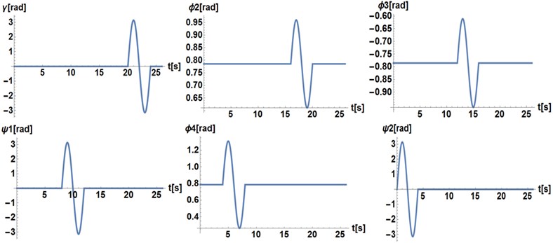
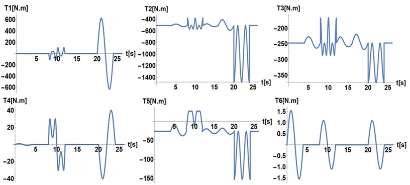
In this simulation, the proposed trajectory consists of a single sinusoidal motion of a period equal to 4 s for each generalized angular coordinate, as shown in Fig. 2. The proposed amplitude for the time series of the generalized coordinates $γ$ , $ψ_{1}$ and $ψ_{2}$ is equal to $π$ rad. For the generalized coordinates $ϕ_{2}$ and $ϕ_{3}$ , the proposed amplitude is $π$ /18 rad. Finally, for the angle $ϕ_{4}$ , the proposed amplitude is $π$ /6. Fig. 3 illustrates the required torques obtained from the inverse dynamics simulation performed.

Fig. 3Theoretical time series of the torques required

4. Conclusions

Maggi’s equations were used to derive a complete non-linear model for the dynamics of 6 degrees of freedom mechanism.

The use of redundant generalized coordinates, led to a significant simplification in the terms related to kinetic and potential energy, which led to a much less complex derivation when compared to the conventional Lagrangian approach.

The use of Baumgarte method avoid the presence of numerical instability associated with the violation of constraints equations during numerical integration.

Finally, the approach applied here to obtain the differential equations of motion might be useful in the dynamic modeling of many other multiple-degree-of-freedom multibody systems.

References

Orsino R. M. M. A Contribution on Modeling Methodologies for Multibody Systems. Ph.D. Thesis, Universidade de São Paulo, Brazil, 2016.

Search CrossRef
Lalusa A., Bauchau O. A. Review of Classical Approaches for Constraint Enforcement in Multibody Systems. Georgia Institute of Technology, 2007.

Publisher
Jinjie W., Guohua C., Zhencai Z., Weihong P., Jishun L. Lateral and torsional vibrations of cable-guided hoisting system with eccentric load. Journal of Vibroengineering, Vol. 18, Issue 6, 2016, p. 3524-3538.

Publisher
Baumgarte J. Stabilization of constraints and integrals of motion in dynamical systems. Computer Methods in Applied Mechanics and Engineering, Vol. 1, 1972, p. 1-16.

Publisher
Malvezzi F., Orsino R. M. M., Coelho T. A. H. Lagrange’s, Maggi’s and Kane’s equations to the dynamic modelling of serial manipulator. Proceedings of DINAME, 2017, https://doi.org/10.1007/978-3-319-91217-2_20.

Publisher
Orsino R. M. M., Hess Coelho T. A., Pesce C. P. Analytical mechanics approaches in the dynamic modelling of Delta mechanism. Robotica, Vol. 33, Issue 4, 2015, p. 953-973.

Publisher

Cited by

Blucher Engineering Proceedings

Beatriz Golin ARCENCIO | Clayton Barcelos ZABEU | Fernando MALVEZZI

(2023)

About this article

Received

01 February 2020

Accepted

10 March 2020

Published

29 June 2020

SUBJECTS

Mathematical models in engineering

DOI

https://doi.org/10.21595/vp.2020.21323

Keywords

Maggi’s equation

multibody dynamics

analytical mechanics

Acknowledgements

Fernando Malvezzi and Renato Maia Matarazzo Orsino acknowledge grant #2018/12087-7, São Paulo Research Foundation (FAPESP).

This is an open access article distributed under the Creative Commons Attribution License, which permits unrestricted use, distribution, and reproduction in any medium, provided the original work is properly cited.

Previous article in issue Previous Next article in issue Next

Research article

2023 10 31

Rigid-flexible coupling modeling of the dual-rotor system for aero-engine

Pingping Ma, Yuehui Dong, Hangqi Zhao, Yang Li, Muge Liu

Research article

2023 05 18

Dynamic modeling and analysis of a vibration-driven robot driven by a conical dielectric elastomer actuator

Xiaojian Wang, Hongguang Li

Research article

2018 12 31

Dynamic modeling and simulation of three-member robot manipulator

Hristijan Mickoski, Ivan Mickoski, Marjan Djidrov

Research article

2017 12 31

Rigid-flexible coupling dynamics simulation of planetary gear transmission based on MFBD

Chiyu Hao, Guangbin Feng, Huagang Sun, Haiping Li

A. Horn, F. Malvezzi, and R. M. M. Orsino, “On the use of Maggi’s equation in the dynamic modeling of multibody systems,” Vibroengineering PROCEDIA, Vol. 32, pp. 166–171, Jun. 2020, https://doi.org/10.21595/vp.2020.21323

Copy Extrica

Copied to clipboard!

TY  - JOUR
DO  - 10.21595/vp.2020.21323
UR  - https://doi.org/10.21595/vp.2020.21323
TI  - On the use of Maggi’s equation in the dynamic modeling of multibody systems
T2  - Vibroengineering PROCEDIA
AU  - Horn, Arthur
AU  - Malvezzi, Fernando
AU  - Orsino, Renato M. M.
PY  - 2020
DA  - 2020/06/29
PB  - JVE International Ltd.
SP  - 166-171
VL  - 32
SN  - 2345-0533
SN  - 2538-8479
ER  - 

Copy Ris

Copied to clipboard!

@article{Horn_2020,
	doi = {10.21595/vp.2020.21323},
	url = {https://doi.org/10.21595/vp.2020.21323},
	year = 2020,
	month = {jun},
	publisher = {{JVE} International Ltd.},
	volume = {32},
	pages = {166--171},
	author = {Arthur Horn and Fernando Malvezzi and Renato M. M. Orsino},
	title = {On the use of Maggi's equation in the dynamic modeling of multibody systems},
	journal = {Vibroengineering {PROCEDIA}}
}

Copy Bibtex

Copied to clipboard!

[1]A. Horn, F. Malvezzi, and R. M. M. Orsino, “On the use of Maggi’s equation in the dynamic modeling of multibody systems,” Vibroengineering PROCEDIA, vol. 32, pp. 166–171, Jun. 2020, doi: 10.21595/vp.2020.21323.

Copy IEEE

Copied to clipboard!

Horn, Arthur, Fernando Malvezzi, and Renato M. M. Orsino. “On the Use of Maggi’s Equation in the Dynamic Modeling of Multibody Systems.” Vibroengineering PROCEDIA 32 (June 29, 2020): 166–71. https://doi.org/10.21595/vp.2020.21323.

Copy Chicago

Copied to clipboard!

On the use of Maggi’s equation in the dynamic modeling of multibody systems

Abstract

Highlights

1. Introduction

2. Differential equation of motion

2.1. Mechanical system

2.2. Mathematical modeling

2.2.1. Notation

2.2.2. Constraints

2.2.3. Stabilization of constraints

2.2.4. Kinematics

2.2.5. Kinetic energy

2.2.6. Potential energy

2.2.7. Generalized forces

2.2.8. Differential equations of motion

3. Numerical simulations

4. Conclusions

References

Cited by

About this article

Related Articles