Dynamics of a single mass vibrating system impacting into a deformable support

Ragulskis, K.; Ragulskis, L.

doi:10.21595/mme.2020.21398

Mathematical Models in Engineering

Browse Journal

Submit article

Published: 31 March 2020

Check for updates

Dynamics of a single mass vibrating system impacting into a deformable support

K. Ragulskis¹

L. Ragulskis²

¹Kaunas University of Technology, K. Donelaičio Str. 73, LT-44249, Kaunas, Lithuania

²Vytautas Magnus University, Vileikos Str. 8, LT-44404, Kaunas, Lithuania

Corresponding Author:

K. Ragulskis

Cite the article Download PDF

Downloads 1090

Abstract

The investigated system comprises a mass attached by a deformable link to a fixed foundation, and an elastic-dissipative limiter of motion of that mass. Such types of systems are widely used in different technological devices and machines. This paper is devoted for the improvement of dynamical qualities of such systems. Free and forced stationary harmonic vibrations as well as the qualitative parameters of motions of the system are analyzed in this paper. Characteristics of vibrations are determined using analytical and numerical techniques. It is determined that for the case of zero fastening the values of eigenfrequencies of the system do not depend on the amplitude of excitation. Then the system has an infinite number of multiple eigenfrequencies. In the case of forced harmonic excitation single valued stable motions exist in the vicinity of the resonance. This gives rise to some qualities of the system which are useful in practical applications.

1. Introduction

This paper is focused on a nonlinear system which is characterized by two following features: first – the values of eigenfrequencies do not depent on the amplitude of excitation, and the second – an infinite number of eigenfrequencies does exist. The dynamics of such kind of systems has not been investigated in the existing literature.

Essentially nonlinear systems, two-dimensional transmissions, their dynamics and vibrations are analysed in [1]. Dynamics of vibromotors for precision microrobots is described in [2]. Resonances in nonlinear vibrating systems are investigated in [3]. Impact dynamics under periodic and transient excitations are analysed in [4]. Stabilization of periodic nonlinear systems is investigated in [5]. Analysis of behaviour of mechanical systems with impacts is performed in [6]. Periodic orbits of mechanical systems with impacts are analysed in [7]. Behaviour of a vibro-impact nonlinear energy sink is investigated in [8]. The dynamics of a particle impact with a wall is analysed in [9].

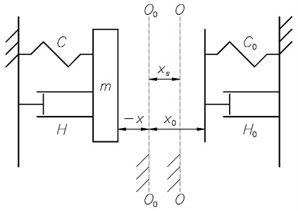
The investigated system is shown in Fig. 1, where $m$ , $C$ and $H$ are the mass of the main vibrating part, the coefficients of stiffness and of viscous friction respectively; while $C_{0}$ and $H_{0}$ are the coefficients of stiffness and viscous friction of the limiter. The positions $O O$ and $O_{0} O_{0}$ are positions of static equilibrium of the contact surfaces of the main part $x$ and of the limiter $x_{0}$ respectively. By $x_{s}$ the fastening of the system in the statical position is denoted. Positive values of $x$ and $x_{0}$ are counted to the right from the position $O_{0} O_{0}$ .

The investigated system is described by the following differential equations:

1

\ddot{x} + (h + h_{0}) \dot{x} + (p^{2} + p_{0}^{2}) x - p^{2} x_{s} = f s i n ω t, x \geq x_{0},

2

\ddot{x} + h \dot{x} + p^{2} x - p^{2} x_{s} = f s i n ω t, x < x_{0},

3

h {\dot{x}}_{0} + p_{0}^{2} x_{0} = 0, x < x_{0},

where:

4

h = \frac{H}{m}, h_{0} = \frac{H_{0}}{m}, p^{2} = \frac{C}{m}, p_{0}^{2} = \frac{C_{0}}{m}, f = \frac{F}{m}, \dot{} = \frac{d}{d t} .

Known methods are used for analytical and numerical investigations.

Fig. 1Schematic representation of the system

2. Free damped vibrations, that is when $x_{s} = f = 0$

Case $x = x_{0},$ that is according to Eq. (1) it is assumed that this takes place in the interval:

5

t \in [0, T_{a}),

and at $t = 0 : x = 0$ , $\dot{x} = {\dot{x}}^{-}$ , and at $t = T_{a}$ goes from the position $x = x_{0}$ to the position $x < x_{0}$ and:

6

\ddot{x} + 2 (h + h_{0}) \dot{x} + (p^{2} + p_{0}^{2}) x = 0,

has the solution:

7

x = C_{1} e^{λ_{1} t} + C_{2} e^{λ_{2} t},

where:

8

λ^{2} + 2 (h + h_{0}) λ + (p^{2} + p_{0}^{2}) = 0,

λ_{1,2} = - (h + h_{0}) \pm i \sqrt{p^{2} + p_{0}^{2} - {(h + h_{0})}^{2}}, i = \sqrt{- 1},

x = e^{- (h + h_{0}) t} (C_{1} c o s \sqrt{} t + C_{2} s i n \sqrt{} t),

where it is denoted:

9

\sqrt{} = \sqrt{p^{2} + p_{0}^{2} - {(h + h_{0})}^{2}} .

$C_{1}$ and $C_{2}$ are found from the initial conditions of motion Eq. (7) at $t = 0 :$

10

0 = e^{- (h + h_{0}) \cdot 0} C_{1} c o s \sqrt{0} \Rightarrow C_{1} = 0,

11

{\dot{x}}^{-} = e^{- (h + h_{0}) t} C_{2} [- (h + h_{0}) s i n \sqrt{} t + \sqrt{} c o s \sqrt{} t] = C_{2} \sqrt{} \Rightarrow C_{2} = \frac{{\dot{x}}^{-}}{\sqrt{}} .

That is:

12

x = \frac{{\dot{x}}^{-}}{\sqrt{}} e^{- (h + h_{0}) t} s i n \sqrt{} t,

13

\dot{x} = e^{- (h + h_{0}) t} \frac{{\dot{x}}^{-}}{\sqrt{}} [- (h + h_{0}) s i n \sqrt{} t + \sqrt{} c o s \sqrt{} t],

14

\ddot{x} = \frac{{\dot{x}}^{-}}{\sqrt{}} e^{- (h + h_{0}) t} [{(h + h_{0})}^{2} s i n \sqrt{} t - (h + h_{0}) \sqrt{} c o s \sqrt{} t - (h + h_{0}) \sqrt{} c o s \sqrt{} t - {(\sqrt{})}^{2} s i n \sqrt{} t],

\ddot{x} = \frac{{\dot{x}}^{-}}{\sqrt{}} e^{- (h + h_{0}) t} \{[{(h + h_{0})}^{2} - {(\sqrt{})}^{2}] s i n \sqrt{} t - 2 (h + h_{0}) \sqrt{} c o s \sqrt{} t\} .

At $t = T_{a}$ the Eq. (3) is not valid and Eqs. (2) and (5) are valid: into Eq. (2) solutions Eqs. (12) and (13) are substituted by assuming $t = T_{a}$ , that is the moment of disconnection of $x$ and $x_{0} :$

15

\ddot{x} + 2 h \dot{x} + p^{2} x = \frac{{\dot{x}}^{-}}{\sqrt{}} e^{- (h + h_{0}) T_{a}} \{[{(h + h_{0})}^{2} - {(\sqrt{})}^{2}] s i n \sqrt{} T_{a} - 2 (h + h_{0}) \sqrt{} c o s \sqrt{} T_{0}

+ 2 h [- (h + h_{0}) s i n \sqrt{} T_{a} + \sqrt{} c o s \sqrt{} T_{a}] + p^{2} s i n \sqrt{} T_{a}\}

= \frac{{\dot{x}}^{-}}{\sqrt{}} e^{- (h + h_{0}) T_{a}} \{[{(h + h_{0})}^{2} - {(\sqrt{})}^{2} - 2 h (h + h_{0}) + p^{2}] s i n \sqrt{} T_{a}

+ [- 2 (h + h_{0}) + 2 h] \sqrt{} c o s \sqrt{} T_{a}\}

= \frac{{\dot{x}}^{-}}{\sqrt{}} e^{- (h + h_{0}) T_{a}} \{[{(h + h_{0})}^{2} - (p^{2} + p_{0}^{2}) + {(h + h_{0})}^{2} - 2 h (h + h_{0}) + p^{2}] s i n \sqrt{} T_{a}

- 2 h_{0} \sqrt{} c o s \sqrt{} T_{a}\}

= \frac{{\dot{x}}^{-}}{\sqrt{}} e^{- (h + h_{0}) T_{a}} \{[- p_{0}^{2} + 2 h_{0} (h + h_{0})] s i n \sqrt{} T_{a} - 2 h_{0} \sqrt{} c o s \sqrt{} T_{a}\} = 0

\Rightarrow t a n \sqrt{} T_{a} = - \frac{2 h_{0} \sqrt{}}{p_{0}^{2} - 2 h_{0} (h + h_{0})} .

The same $T_{a}$ must be obtained by substituting the solutions $\dot{x}$ and $x$ at $T_{a}$ into Eq. (1), that is:

2 h_{0} {\dot{x}}_{0} + {p_{0}^{2} x_{0}|}_{{x = x_{0}|}_{t = T_{a}}} \equiv - 2 h_{0} (h + h_{0}) s i n \sqrt{} T_{a} + 2 h_{0} \sqrt{} c o s \sqrt{} T_{a} + p_{0}^{2} s i n \sqrt{} T_{a} = 0

\Rightarrow t a n \sqrt{} T_{a} = - \frac{2 h_{0} \sqrt{}}{p_{0}^{2} - 2 h_{0} (h + h_{0})} .

Further at $t \in (T_{a}, T_{k})$ motion takes place according to the Eqs. (2) and (3) with initial parameters:

16

x (T_{a}) = \frac{{\dot{x}}^{-}}{\sqrt{}} e^{- (h + h_{0}) T_{a}} s i n \sqrt{} T_{a}, \dot{x} (T_{a}) = \frac{{\dot{x}}^{-}}{\sqrt{}} e^{- (h + h_{0}) T_{a}} [- (h + h_{0}) s i n \sqrt{} T_{a} + \sqrt{} c o s \sqrt{} T_{a}] .

The solution of Eq. (2) in the interval:

17

t \in (T_{a}, T_{0}),

where:

18

x (T_{0}) = 0, \dot{x} (T_{0}) = {\dot{x}}^{+} (T_{0}),

is:

19

x = e^{- h (t - T_{a})} [D_{1} c o s \sqrt{p^{2} - h^{2}} (t - T_{a}) + D_{2} s i n \sqrt{p^{2} - h^{2}} (t - T_{a})],

where $D_{1}$ , $D_{2}$ are found according to the initial conditions Eq. (14):

20

x (T_{a}) = D_{1},

\dot{x} (T_{a}) = - h D_{1} c o s \sqrt{p^{2} - h^{2}} 0 - h \sqrt{p^{2} - h^{2}} D_{2} s i n \sqrt{p^{2} - h^{2}} 0

- D_{2} \sqrt{p^{2} - h^{2}} c o s 0 = - D_{1} h - D_{2} \sqrt{p^{2} - h^{2}},

D_{1} = x (T_{0}),

\dot{x} (T_{a}) = - h x (T_{a}) - \sqrt{p^{2} - h^{2}} D_{2} \Rightarrow D_{2} = - \frac{\dot{x} (T_{a})}{\sqrt{p^{2} - h^{2}}} - \frac{h}{\sqrt{p^{2} - h^{2}}} x (T_{a}) .

Eq. (20) minus Eq. (19) gives:

21

x = e^{- h (t - T_{a})} \{x (T_{a}) c o s \sqrt{p^{2} - h^{2}} (t - T_{a})

- \frac{1}{\sqrt{p^{2} - h^{2}}} [h x (T_{a}) + \dot{x} (T_{a})] s i n \sqrt{p^{2} - h^{2}} (t - T_{a})\},

\dot{x} = e^{- h (t - T_{a})} \{- h x (T_{a}) c o s \sqrt{p^{2} - h^{2}} (t - T_{a})

+ \frac{h}{\sqrt{p^{2} - h^{2}}} [h x (T_{a}) + \dot{x} (T_{a})] s i n \sqrt{p^{2} - h^{2}} (t - T_{a})

- x (T_{a}) \sqrt{p^{2} - h^{2}} s i n \sqrt{p^{2} - h^{2}} (t - T_{a}) - [h x (T_{a}) + \dot{x} (T_{a})] c o s \sqrt{p^{2} - h^{2}} (t - T_{a})\}

= e^{- h (t - T_{a})} \{- [2 h x (T_{a}) + \dot{x} (T_{a})] c o s \sqrt{p^{2} - h^{2}} (t - T_{a})

+ [(\frac{h^{2}}{\sqrt{p^{2} - h^{2}}} - \sqrt{p^{2} - h^{2}}) x (T_{a}) + \frac{h}{\sqrt{p^{2} - h^{2}}} \dot{x} (T_{a})] s i n \sqrt{p^{2} - h^{2}} (t - T_{a})\}

= e^{- h (t - T_{a})} \{- [2 h x (T_{a}) + \dot{x} (T_{a})] c o s \sqrt{p^{2} - h^{2}} (t - T_{a})

+ [\frac{- p^{2}}{\sqrt{p^{2} - h^{2}}} x (T_{a}) + \frac{h}{\sqrt{p^{2} - h^{2}}} \dot{x} (T_{a})] s i n \sqrt{p^{2} - h^{2}} (t - T_{a})\},

\dot{x} = e^{- h (t - T_{a})} \{- [2 h x (T_{a}) + \dot{x} (T_{a})] c o s \sqrt{p^{2} - h^{2}} (t - T_{a})

+ \frac{1}{\sqrt{p^{2} - h^{2}}} [- p^{2} x (T_{a}) + h \dot{x} (T_{a})] s i n \sqrt{p^{2} - h^{2}} (t - T_{a})\} .

It is assumed that when $t = T :$

22

x (T) = 0, \dot{x} (T) = {\dot{x}}^{-} (T), T = T_{a} + T_{b} .

In the Eqs. (20), (21) by assuming $t = T,$ that is $t - T_{a} = T_{b} :$

23

0 = e^{- h (T - T_{a})} \{x (T_{a}) c o s \sqrt{p^{2} - h^{2}} (T - T_{a})

- \frac{1}{\sqrt{p^{2} - h^{2}}} [h x (T_{a}) + \dot{x} (T_{a})] s i n \sqrt{p^{2} - h^{2}} (T - T_{a})\},

24

\dot{x} = e^{- h (T - T_{a})} \{- [2 h x (T_{a}) + \dot{x} (T_{a})] c o s \sqrt{p^{2} - h^{2}} (T - T_{a})

+ \frac{1}{\sqrt{p^{2} - h^{2}}} [- p^{2} x (T_{a}) + h \dot{x} (T_{a})] s i n \sqrt{p^{2} - h^{2}} (T - T_{a})\} .

From Eq. (23) $T$ is determined and from Eq. (24) ${\dot{x}}^{-} (T) .$

The coefficient of restitution of velocity of the support is:

25

R_{h} = \frac{\dot{x} (T_{a})}{x^{-}},

by taking into account Eqs. (13) and (15):

26

R_{h} = \frac{e^{- (h + h_{0}) T_{a}}}{\sqrt{}} [- (h + h_{0}) s i n \sqrt{} T_{a} + \sqrt{} c o s \sqrt{} T_{a}],

or:

27

R_{h} = \frac{e^{- (h + h_{0}) T_{a}}}{c o s \sqrt{} T_{a}} \cdot \frac{p_{0}^{2}}{p_{0}^{2} - 2 h_{0} (h + h_{0})},

where $T_{0}$ is determined by the Eq. (15).

3. Vibrations of the conservative system

In this case in the Eqs. (1-3) it is assumed that:

28

h = h_{0} = f = 0, x_{s} > 0 .

Two intervals of time are investigated: the first one:

29

t \in [0, {\bar{T}}_{1}], x = x_{0},

and the second one:

30

t \in [{\bar{T}}_{1}, \bar{T} = T_{1} + T_{2}], x < x_{0} .

In case of the first interval it is assumed:

31

t = 0 : x = x_{0} = 0, \dot{x} = {\dot{x}}^{-} > 0,

32

t = {\bar{T}}_{1} : x = x_{0} = 0, \dot{x} = - {\dot{x}}^{-} .

According to the Eqs. (1), (28), (29), (30) it is obtained:

33

x = - D_{1} c o s \sqrt{p^{2} + p_{0}^{2}} t + D_{2} s i n \sqrt{p^{2} + p_{0}^{2}} t + D_{1},

34

\frac{\dot{x}}{\sqrt{p^{2} + p_{0}^{2}}} = D_{1} s i n \sqrt{p^{2} + p_{0}^{2}} t + D_{2} c o s \sqrt{p^{2} + p_{0}^{2}} t,

where:

35

D_{1} = \frac{p^{2}}{p^{2} + p_{0}^{2}} x_{1}, D_{2} = \frac{{\dot{x}}^{-}}{\sqrt{p^{2} + p_{0}^{2}}} .

At $t = {\bar{T}}_{1}$ , by taking into account Eqs. (32-35), it is obtained:

36

t a n \sqrt{p^{2} + p_{0}^{2}} {\bar{T}}_{1} = \frac{2 X_{s}}{1 - X_{s}^{2}},

where:

37

X_{s} = \frac{1}{\sqrt{1 + {(\frac{p_{0}}{p})}^{2}}} \cdot \frac{p x_{s}}{{\dot{x}}^{-}} .

In case of the second interval by taking into account Eq. (30) it is assumed:

38

t = {\bar{T}}_{1} : x = x_{0}, \dot{x} = - {\dot{x}}^{-},

39

t = {\bar{T}}_{1} + {\bar{T}}_{2} : x = x_{0}, \dot{x} = {\dot{x}}^{-} .

According to the Eqs. (2), (28), (38), (39) it is obtained:

40

x = - x_{s} c o s p (t - {\bar{T}}_{1}) - \frac{{\dot{x}}^{-}}{p} s i n (t - {\bar{T}}_{1}) + x_{s},

41

\frac{\dot{x}}{\bar{p}} = x_{s} s i n p (t - T_{1}) - \frac{{\dot{x}}^{-}}{p} c o s p (t - {\bar{T}}_{1}) .

At $t = {\bar{T}}_{1} + {\bar{T}}_{2},$ by taking into account Eqs. (39-41), it is obtained:

42

t a n p {\bar{T}}_{2} = 2 \frac{\frac{p x_{s}}{ω}}{(\frac{p x_{s}}{{\dot{x}}^{-}}) - 1} .

Period of the system:

43

\bar{T} = {\bar{T}}_{1} + {\bar{T}}_{2},

where ${\bar{T}}_{1}$ and ${\bar{T}}_{2}$ are determined according to the Eqs. (36), (37), (42).

In separate case, when:

44

x_{s} = 0,

according to the Eqs. (36), (37), (42) it is obtained:

45

{\bar{T}}_{1} = \frac{π}{p}, {\bar{T}}_{2} = \frac{π}{p \sqrt{1 + {(\frac{p_{0}}{p})}^{2}}},

that is:

46

T = [1 + \frac{1}{\sqrt{1 + {(\frac{p_{0}}{p})}^{2}}}] \frac{π}{p} .

4. Numerical investigation of the damped system

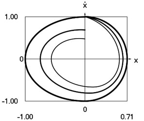
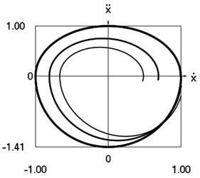
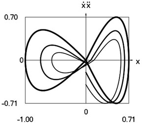
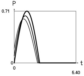
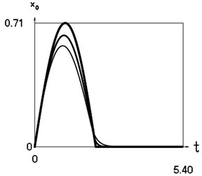
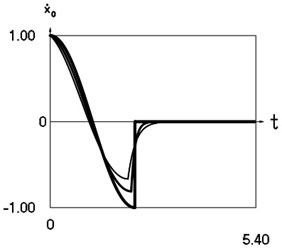
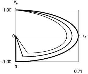
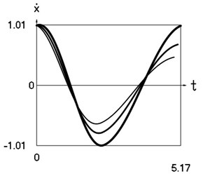
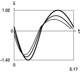
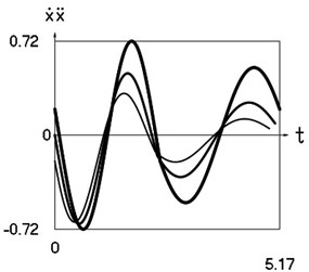
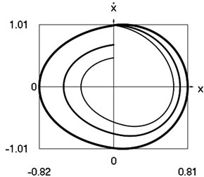
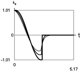
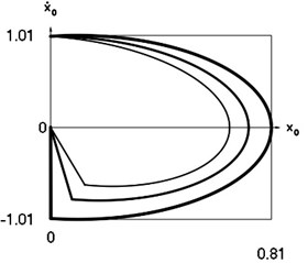
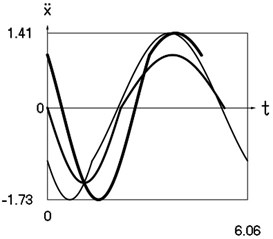
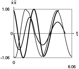
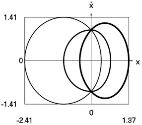
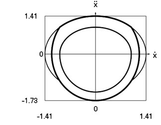
It is assumed that $x (0) = 0$ , $\dot{x} (0) = 1$ , $x_{0} (0) = 0$ , $c = 1$ , $c_{0} = 1 .$ Results for $h = h_{0} =$ 0.2 are represented by a thin line; for $h = h_{0} =$ 0.1 are represented by a line of medium thickness; for $h = h_{0} =$ 0.001 are represented by a thick line. The force is calculated as $P = h_{0} {\dot{x}}_{0} + c_{0} x_{0} .$

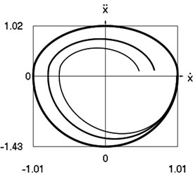
Results of computations at $x_{s} =$ –0.2 are depicted in Fig. 2.

Fig. 2Dynamics of the system at xs= –0.2

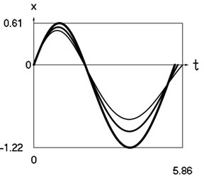
a) Displacement as function of time

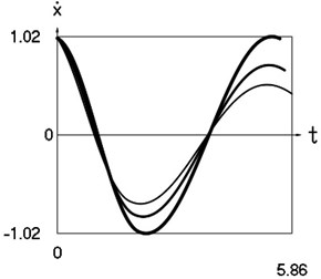
b) Velocity as function of time

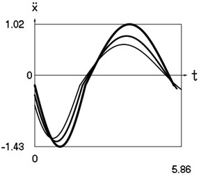
c) Acceleration as function of time

d) Velocity multiplied by acceleration as function of time

e) Phase trajectory: velocity as function of displacement

f) Phase trajectory: acceleration as function of velocity

g) Phase trajectory: velocity multiplied by acceleration as function of displacement

h) Force as function of time

i) Displacement of support as function of time

j) Velocity of support as function of time

k) Phase trajectory: velocity of support as function of displacement of support

Analogously, results of computations at $x_{s} = 0$ are depicted in Fig. 3.

Fig. 3Dynamics of the system at xs=0

a) Displacement as function of time

b) Velocity as function of time

c) Acceleration as function of time

d) Velocity multiplied by acceleration as function of time

e) Phase trajectory: velocity as function of displacement

f) Phase trajectory: acceleration as function of velocity

g) Phase trajectory: velocity multiplied by acceleration as function of displacement

h) Force as function of time

i) Displacement of support as function of time

j) Velocity of support as function of time

k) Phase trajectory: velocity of support as function of displacement of support

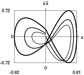
Finally, results of computations at $x_{s} =$ 0.2 are depicted in Fig. 4.

Fig. 4Dynamics of the system at xs= 0.2

a) Displacement as function of time

b) Velocity as function of time

c) Acceleration as function of time

d) Velocity multiplied by acceleration as function of time

e) Phase trajectory: velocity as function of displacement

f) Phase trajectory: acceleration as function of velocity

g) Phase trajectory: velocity multiplied by acceleration as function of displacement

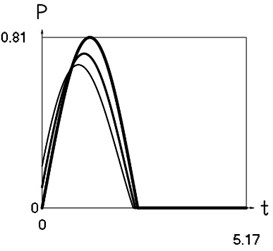
h) Force as function of time

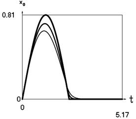
i) Displacement of support as function of time

j) Velocity of support as function of time

k) Phase trajectory: velocity of support as function of displacement of support

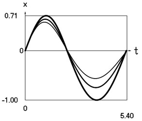
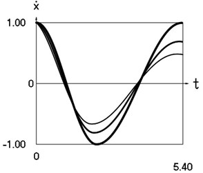
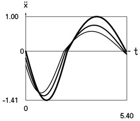
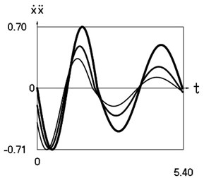
5. Numerical investigation of the conservative system

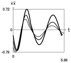
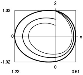
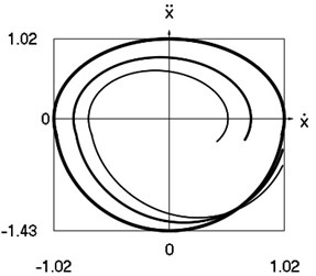
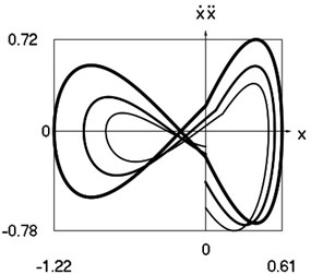
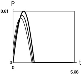
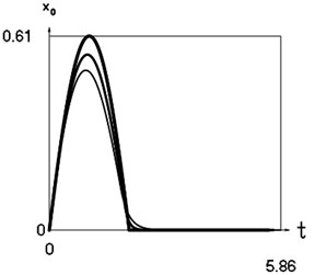
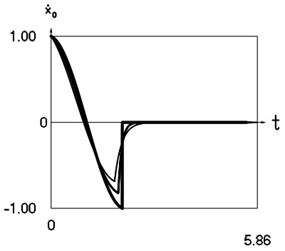
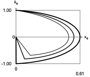
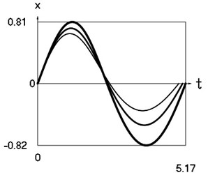
It is assumed that $x (0) =$ 0, $\dot{x} (0) =$ 1, $c =$ 1, $c_{0} =$ 1. Results for $x_{s} =$ –1 are represented by a thin line; for $x_{s} = 0$ are represented by a line of medium thickness; for $x_{s} =$ 1 are represented by a thick line. The force is calculated as $P = c_{0} x_{0} .$

Fig. 5The dynamics of the conservative system

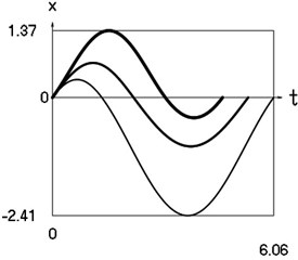
a) Displacement as function of time

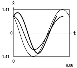
b) Velocity as function of time

c) Acceleration as function of time

d) Velocity multiplied by acceleration as function of time

e) Phase trajectory: velocity as function of displacement

f) Phase trajectory: acceleration as function of velocity

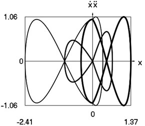
g) Phase trajectory: velocity multiplied by acceleration as function of displacement

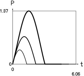
h) Force as function of time

Simulation results for the investigated system are presented in Fig. 5.

6. Conclusions

Essentially nonlinear vibro-impact systems may have a number of various regimes of motion in steady state regimes under harmonic excitation. That couses unstable operation of such types of systems. Small variations of parameters or excitation jumps from one type of regime to another type of regime may occur. The purpose of this paper is to avoid this disadvantage in the behaviour of such system. This is achieved by choosing the fastening (the difference in the positions of statical equilibrium of impacting surfaces) between impacting members of the system to be equal to zero. All this is shown by the obtained formulas and graphical relationships, which were obtained by analytical and numerical methods.

On the basis of the presented results the qualities of dynamic behavior of the investigated essentially nonlinear vibrating system are revealed. Analytical relationships describing the motion of the system have been determined and are presented in the paper. Free damped vibrations, vibrations of the conservative system, time histories of motion as well as phase trajectories of motion for typical values of system parameters are presented in detail.

That opens a potential for the applicability of such systems in a wide variety of engineering applications.

References

Kurila R., Ragulskienė V. Two-Dimensional Vibro-Transmissions. Mokslas, Vilnius, 1986, (in Russian).

Search CrossRef
Ragulskis K., Bansevičius R., Barauskas R., Kulvietis G. Vibromotors for Precision Microrobots. Hemisphere, New York, 1987.

Search CrossRef
Wedig W. V. New resonances and velocity jumps in nonlinear road-vehicle dynamics. Procedia IUTAM, Vol. 19, 2016, p. 209-218.

Publisher
Li T., Gourc E., Seguy S., Berlioz A. Dynamics of two vibro-impact nonlinear energy sinks in parallel under periodic and transient excitations. International Journal of Non-Linear Mechanics, Vol. 90, 2017, p. 100-110.

Publisher
Zaitsev V. A. Global asymptotic stabilization of periodic nonlinear systems with stable free dynamics. Systems and Control Letters, Vol. 91, 2016, p. 7-13.

Publisher
Dankowicz H., Fotsch E. On the analysis of chatter in mechanical systems with impacts. Procedia IUTAM, Vol. 20, 2017, p. 18-25.

Publisher
Spedicato S., Notarstefano G. An optimal control approach to the design of periodic orbits for mechanical systems with impacts. Nonlinear Analysis: Hybrid Systems, Vol. 23, 2017, p. 111-121.

Search CrossRef
Li W., Wierschem N. E., Li X., Yang T. On the energy transfer mechanism of the single-sided vibro-impact nonlinear energy sink. Journal of Sound and Vibration, Vol. 437, 2018, p. 166-179.

Publisher
Marshall J. S. Modeling and sensitivity analysis of particle impact with a wall with integrated damping mechanisms. Powder Technology, Vol. 339, 2018, p. 17-24.

Publisher

About this article

Received

27 December 2019

Accepted

24 March 2020

Published

31 March 2020

DOI

https://doi.org/10.21595/mme.2020.21398

Keywords

limiter of motion

conservative system

natural frequencies

forced motions

This is an open access article distributed under the Creative Commons Attribution License, which permits unrestricted use, distribution, and reproduction in any medium, provided the original work is properly cited.

Previous article in issue Previous

Research article

2023 06 25

Vibrator with two impacting pairs, one of them in the position of equilibrium

K. Ragulskis, L. Ragulskis

Research article

2021 12 02

Mathematical modeling of forced oscillations of semidefinite vibro-impact system sliding along rough horizontal surface

Vitaliy Korendiy, Volodymyr Gursky, Oleksandr Kachur, Volodymyr Gurey, Oleksandr Havrylchenko, Oleh Kotsiumbas

Research article

2021 06 30

Investigation of single valued motions in the vibro-impact system in case of harmonic force

K. Ragulskis, L. Ragulskis

Research article

2021 06 28

Mathematical modelling of forced oscillations of continuous members of resonance vibratory system

Oleksandr Kachur, Oleksii Lanets, Vitaliy Korendiy, Vasyl Lozynskyy, Oleh Kotsiumbas, Oleksandr Havrylchenko, Nadiia Maherus

K. Ragulskis and L. Ragulskis, “Dynamics of a single mass vibrating system impacting into a deformable support,” Mathematical Models in Engineering, Vol. 6, No. 1, pp. 66–78, Mar. 2020, https://doi.org/10.21595/mme.2020.21398

Copy Extrica

Copied to clipboard!

TY  - JOUR
DO  - 10.21595/mme.2020.21398
UR  - https://doi.org/10.21595/mme.2020.21398
TI  - Dynamics of a single mass vibrating system impacting into a deformable support
T2  - Mathematical Models in Engineering
AU  - Ragulskis, K.
AU  - Ragulskis, L.
PY  - 2020
DA  - 2020/03/31
PB  - JVE International Ltd.
SP  - 66-78
IS  - 1
VL  - 6
SN  - 2351-5279
SN  - 2424-4627
ER  - 

Copy Ris

Copied to clipboard!

@article{Ragulskis_2020,
	doi = {10.21595/mme.2020.21398},
	url = {https://doi.org/10.21595/mme.2020.21398},
	year = 2020,
	month = {mar},
	publisher = {{JVE} International Ltd.},
	volume = {6},
	number = {1},
	pages = {66--78},
	author = {K. Ragulskis and L. Ragulskis},
	title = {Dynamics of a single mass vibrating system impacting into a deformable support},
	journal = {Mathematical Models in Engineering}
}

Copy Bibtex

Copied to clipboard!

[1]K. Ragulskis and L. Ragulskis, “Dynamics of a single mass vibrating system impacting into a deformable support,” Mathematical Models in Engineering, vol. 6, no. 1, pp. 66–78, Mar. 2020, doi: 10.21595/mme.2020.21398.

Copy IEEE

Copied to clipboard!

Ragulskis, K., and L. Ragulskis. “Dynamics of a Single Mass Vibrating System Impacting into a Deformable Support.” Mathematical Models in Engineering 6, no. 1 (March 31, 2020): 66–78. https://doi.org/10.21595/mme.2020.21398.

Copy Chicago

Copied to clipboard!

Dynamics of a single mass vibrating system impacting into a deformable support

Abstract

1. Introduction

2. Free damped vibrations, that is when xs=f=0

3. Vibrations of the conservative system

4. Numerical investigation of the damped system

5. Numerical investigation of the conservative system

6. Conclusions

References

About this article

Related Articles

2. Free damped vibrations, that is when $x_{s} = f = 0$