Investigation of single valued motions in the vibro-impact system in case of harmonic force

1. Introduction

In practical applications in engineering various dynamic regimes of motion of vibro-impact systems take place. An important problem is to investigate those regimes of motion, which are used in engineering applications.

In this paper dynamics in some typical regimes of motion are investigated in detail. Vibrations excited by a force of the system performing vibrations with impacts with excitation by a harmonic force are analysed. Graphical results of investigation for the values of parameters which are typical for the vibrating system were obtained and are shown in detail.

The results of investigation are used in the process of design of systems performing vibrations with impacts and they are applied in different types of technological processes and machines of different types.

Investigation of resonances in vehicle dynamics is presented in [1]. Impacts under periodic and transient excitations are investigated in [2]. Problem of stabilisation of periodic nonlinear systems is solved in [3]. Mechanical systems in which impacts take place are investigated in [4]. Periodic orbits in mechanical systems with impacts are presented in [5]. Investigation of the vibro-impact system and the energy transfer mechanism in it is performed in [6]. Analysis of particle impact with a wall is performed in [7]. Frequency analysis of the system performing vibrations is performed in [8]. Investigation of dynamics of a pendulum mechanism is performed in [9]. Systems with piecewise-linear type of nonlinearity are investigated in [10]. Investigation of resonant zones of a dynamical system is performed in [11]. Analysis of the Sommerfeld effect in a nonlinear oscillator is presented in [12]. Investigation of isolated resonances in a dynamical system is performed in [13]. Analysis of vibro-impact mechanism is presented in [14]. All the references are essential in understanding the current status of investigations of essentially nonlinear mechanical systems.

In this paper first of all model of the system performing vibrations with impacts is presented. The obtained results for several typical regimes of motion of the system are investigated and described in detail. Typical frequency regions with single valued regimes of motion are determined.

The presented results of investigation are used for the design of systems performing vibrating motions with impacts as well as mechanisms of various types. In this paper the phenomenon of impact is investigated and it takes place in the process of operation of various types of mechanical systems and mechanisms as well as machines.

2. Model of the investigated vibro-impact system

Dynamics of the system performing vibrations with impacts is governed by the differential equation:

where $m$ denotes the mass, $H$ denotes the viscous damping coefficient, $C$ denotes the stiffness coefficient, $F$ denotes the excitation amplitude, $\omega$ denotes the frequency, $t$ denotes the time variable, the dot above the quantity indicates derivative by t.

Process of impact is described as:

where by $R$ the restitution coefficient is denoted, by superscript minus the quantity before impact is denoted, by superscript plus the quantity after impact is denoted.

In non dimensional form Eq. (1) becomes:

In non dimensional form Eq. (2) becomes:

In the performed investigations the exciting force is denoted as:

Motions of the system in regimes that are periodic are investigated and the following graphical representations are presented: $\stackrel{-}{f}$ as function of $\tau ,$$x$ as function of $\tau ,$$x\text{'}$ as function of $\tau ,$$x\text{'}$ as function of $x.$

Further vibrations of the vibro impact system for several typical regimes of motions performing steady state vibrations are investigated.

3. Dynamics in periodic regimes of motion for low frequency of excitation

Graphical relationships for three typical values of $\nu$ are shown in the Figs. 1, 2 and 3 in order of increasing values of $\nu .$

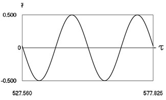
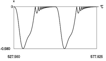
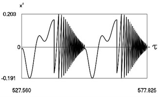
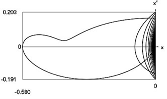
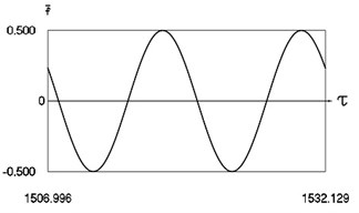
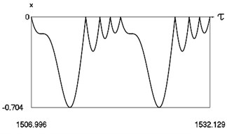
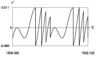
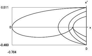
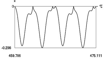
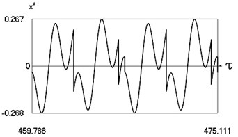
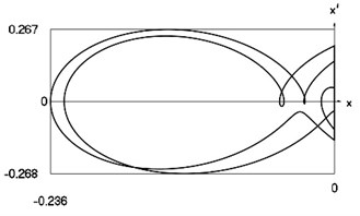
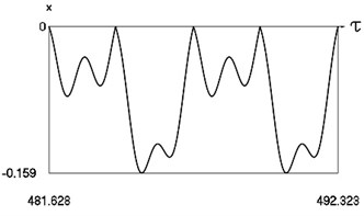
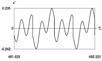
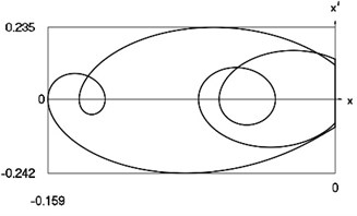
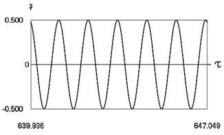
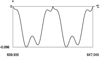
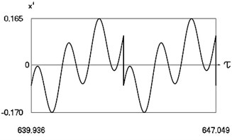
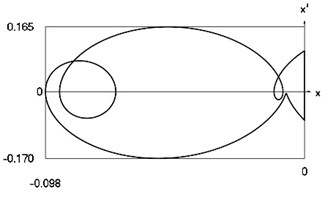
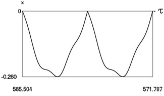
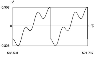
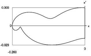
Fig. 1 shows variation of force in time, variation of displacement in time, variation of velocity in time and variation of velocity as function of displacement for $\nu =1/6.$ It is seen that a very great number of multiple very fastly decaying impacts take place.

Fig. 2 shows variation of force in time, variation of displacement in time, variation of velocity in time and variation of velocity as function of displacement for $\nu =1/4.$ It is seen that a great number of multiple fastly decaying impacts take place.

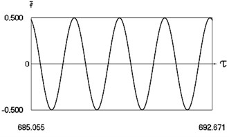
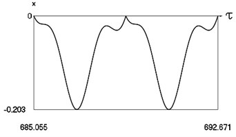
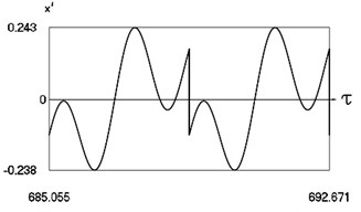
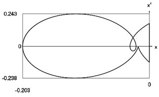
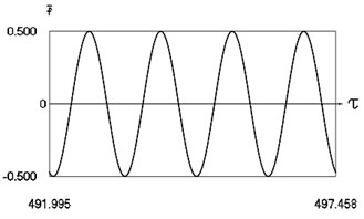
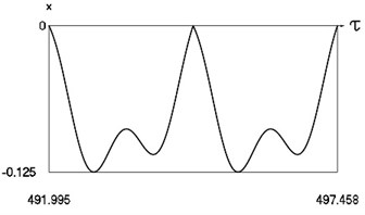
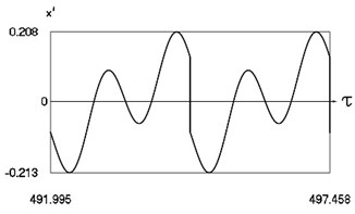
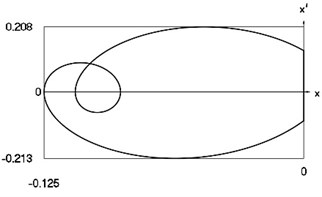
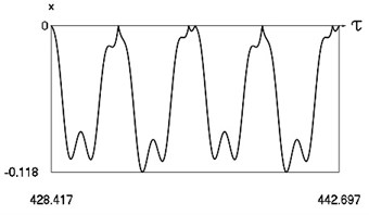
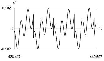
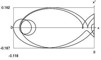
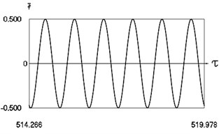
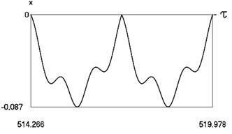
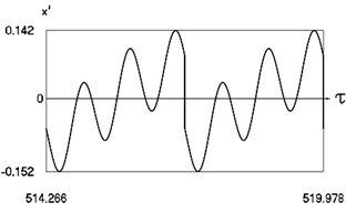
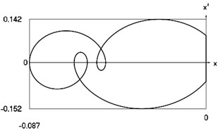
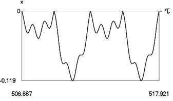
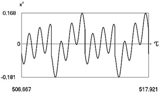
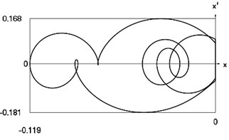
Fig. 3 shows variation of force in time, variation of displacement in time, variation of velocity in time and variation of velocity as function of displacement for $\nu =1/2.$ It is seen that multiple decaying impacts take place.

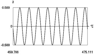
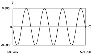
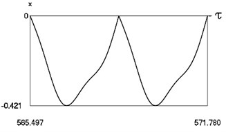
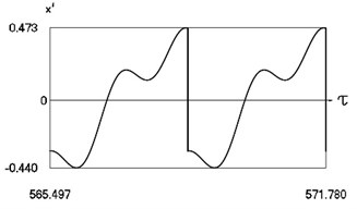
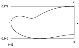
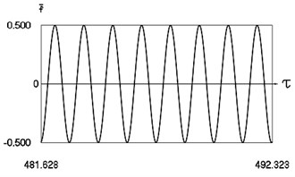
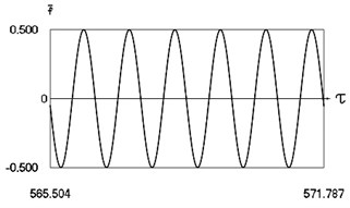
Fig. 1Motion in periodic regime at ν= 1/6, f= –0.5, h= 0.1, R= 0.975

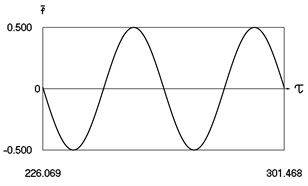
a) Exciting force

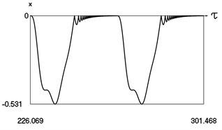
b) Variation of displacement

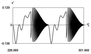
c) Variation of velocity

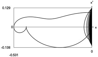
d) Relationship between velocity of the system and its displacement

Fig. 2Motion in periodic regime at ν= 1/4, f= –0.5, h= 0.1, R= 0.94

a) Exciting force

b) Variation of displacement

c) Variation of velocity

d) Relationship between velocity of the system and its displacement

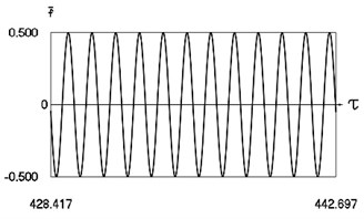
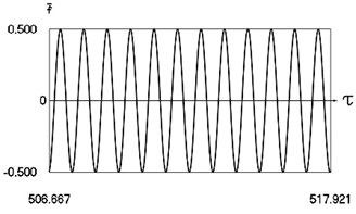
Fig. 3Motion in periodic regime at ν= 1/2, f= –0.5, h= 0.1, R= 0.9

a) Exciting force

b) Variation of displacement

c) Variation of velocity

d) Relationship between velocity of the system and its displacement

It is observed that during the motion in a period of force a number of impacts are observed. With the value of $\nu$ becoming smaller in general the number of impacts becomes higher. Decaying impacts are clearly observed in the obtained results. Thus it can be considered that cyclic motion of the vibro-impact system takes place.

4. Dynamics in periodic regimes of motion for frequency around four

Graphical relationships for five typical values of $\nu$ are shown in the Figs. 4-8. The first Figure is near to the region of single valued motions from the external side of this region, while the second Figure is near to the region of single valued motions from the internal side and thus they approximately represent the lower boundary of the region of single valued motions. The third Figure represents motion at the approximately optimal frequency of excitation. The fourth Figure is near to the region of single valued motions from the internal side of this region, while the fifth Figure is near to the region of single valued motions from the external side and thus they approximately represent the upper boundary of the region of single valued motions.

Fig. 4Motion in periodic regime at ν= 3.28, f= –0.5, h= 0.1, R= 0.7

a) Exciting force

b) Variation of displacement

c) Variation of velocity

d) Relationship between velocity of the system and its displacement

Fig. 4 shows variation of force in time, variation of displacement in time, variation of velocity in time and variation of velocity as function of displacement for $\nu =$ 3.28. It is seen that the system is operating at the lower border outside of the recommended zone of single valued motions.

Fig. 5 shows variation of force in time, variation of displacement in time, variation of velocity in time and variation of velocity as function of displacement for $\nu =$ 3.3. It is seen that the system is operating at the lower border inside of the recommended zone of single valued motions.

Fig. 5Motion in periodic regime at ν= 3.3, f= –0.5, h= 0.1, R= 0.7

a) Exciting force

b) Variation of displacement

c) Variation of velocity

d) Relationship between velocity of the system and its displacement

Fig. 6Motion in periodic regime at ν= 4,6, f= –0.5, h= 0.1, R= 0.7

a) Exciting force

b) Variation of displacement

c) Variation of velocity

d) Relationship between velocity of the system and its displacement

Fig. 6 shows variation of force in time, variation of displacement in time, variation of velocity in time and variation of velocity as function of displacement for $\nu =$ 4. It is seen that the system is operating at recommended frequency.

Fig. 7 shows variation of force in time, variation of displacement in time, variation of velocity in time and variation of velocity as function of displacement for $\nu =$ 4.6. It is seen that the system is operating at the upper border inside of the recommended zone of single valued motions.

Fig. 8 shows variation of force in time, variation of displacement in time, variation of velocity in time and variation of velocity as function of displacement for $\nu =$ 4.7. It is seen that the system is operating at the upper border outside of the recommended zone of single valued motions.

From the obtained graphical relationships the recommended zone of single valued motions can be seen.

Fig. 7Motion in periodic regime at ν= 4.26, f= –0.5, h= 0.1, R= 0.7

a) Exciting force

b) Variation of displacement

c) Variation of velocity

d) Relationship between velocity of the system and its displacement

Fig. 8Motion in periodic regime at ν= 4.7, f= –0.5, h= 0.1, R= 0.7

a) Exciting force

b) Variation of displacement

c) Variation of velocity

d) Relationship between velocity of the system and its displacement

5. Dynamics in periodic regimes of motion for frequency around six

Graphical relationships for five typical values of $\nu$ are shown in the Figs. 9-13. The first Figure is near to the region of single valued motions from the external side of this region, while the second Figure is near to the region of single valued motions from the internal side and thus they approximately represent the lower boundary of the region of single valued motions. The third Figure represents motion at the approximately optimal frequency of excitation. The fourth Figure is near to the region of single valued motions from the internal side of this region, while the fifth Figure is near to the region of single valued motions from the external side and thus they approximately represent the upper boundary of the region of single valued motions.

Fig. 9 shows variation of force in time, variation of displacement in time, variation of velocity in time and variation of velocity as function of displacement for $\nu =$ 5.28. It is seen that the system is operating at the lower border outside of the recommended zone of single valued motions.

Fig. 10 shows variation of force in time, variation of displacement in time, variation of velocity in time and variation of velocity as function of displacement for $\nu =$ 5.3. It is seen that the system is operating at the lower border inside of the recommended zone of single valued motions.

Fig. 9Motion in periodic regime at ν= 5.28, f= –0.5, h= 0.1, R= 0.7

a) Exciting force

b) Variation of displacement

c) Variation of velocity

d) Relationship between velocity of the system and its displacement

Fig. 10Motion in periodic regime at ν= 5.3, f= –0.5, h= 0.1, R= 0.7

a) Exciting force

b) Variation of displacement

c) Variation of velocity

d) Relationship between velocity of the system and its displacement

Fig. 11 shows variation of force in time, variation of displacement in time, variation of velocity in time and variation of velocity as function of displacement for $\nu =$ 6. It is seen that the system is operating at recommended frequency.

Fig. 12 shows variation of force in time, variation of displacement in time, variation of velocity in time and variation of velocity as function of displacement for $\nu =$ 6.6. It is seen that the system is operating at the upper border inside of the recommended zone of single valued motions.

Fig. 13 shows variation of force in time, variation of displacement in time, variation of velocity in time and variation of velocity as function of displacement for $\nu =$ 6.7. It is seen that the system is operating at the upper border outside of the recommended zone of single valued motions.

From the obtained graphical relationships the recommended zone of single valued motions can be seen.

Fig. 11Motion in periodic regime at ν= 6, f= –0.5, h= 0.1, R= 0.7

a) Exciting force

b) Variation of displacement

c) Variation of velocity

d) Relationship between velocity of the system and its displacement

Fig. 12Motion in periodic regime at ν= 6.6, f= –0.5, h= 0.1, R= 0.7

a) Exciting force

b) Variation of displacement

c) Variation of velocity

d) Relationship between velocity of the system and its displacement

Fig. 13Motion in periodic regime at ν= 6.7, f= –0.5, h= 0.1, R= 0.7

a) Exciting force

b) Variation of displacement

c) Variation of velocity

d) Relationship between velocity of the system and its displacement

6. Regions of optimal behavior of the system in periodic regimes of motion

Minimum and maximum values of basic parameters determining dynamic behavior of the investigated vibro-impact system are investigated as functions of frequency of excitation. Frequency regions were minimum and maximum values coincide correspond to regions of single valued motions, while to the left and right of those regions multi valued motions take place. Single valued motions are important in practical applications and thus this paper is devoted to their investigation.

Parameters describing the dynamics at $\nu =$ 2 are shown in Fig. 14.

Fig. 14Minimum values and maximum values for h= 0.1, R= 0.7 in the vicinity of ν= 2

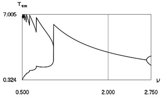
a) Intervals between impacts

b) Derivatives of displacement before the moment of impact

c) Minimum values of displacements in the intervals between impacts

In Fig. 14 the values of intervals between impacts, velocities before impact and minimum values of displacements in the intervals between impacts are represented.

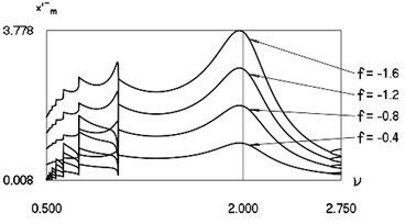
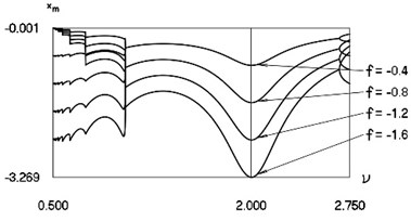
Parameters describing the dynamics at $\nu =$ 4 are shown in Fig. 15.

In Fig. 15 the values of intervals between impacts, velocities before impact and minimum values of displacements in the intervals between impacts are represented.

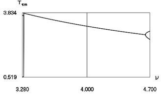
Parameters describing the dynamics at $\nu =$ 6 are shown in Fig. 16.

Fig. 15Minimum values and maximum values for h= 0.1, R= 0.7 in the vicinity of ν= 4

a) Intervals between impacts

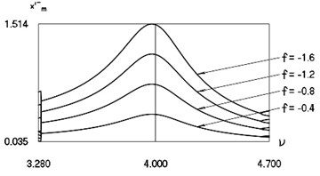
b) Derivatives of displacement before the moment of impact

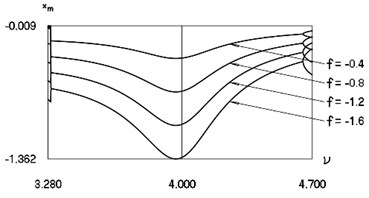
c) Minimum values of displacements in the intervals between impacts

Fig. 16Minimum values and maximum values for h= 0.1, R= 0.7 in the vicinity of ν= 6

a) Intervals between impacts

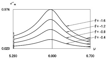
b) Derivatives of displacement before the moment of impact

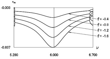
c) Minimum values of displacements in the intervals between impacts

In Fig. 16 the values of intervals between impacts, velocities before impact and minimum values of displacements in the intervals between impacts are represented.

Results at $f=$ –0.4, $f=$ –0.8, $f=$ –1.2, $f=$ –1.6 are presented in the previous three figures. Intervals between impacts are mutually similar for the four values of $f$. Recommended frequency regions are clearly seen in the presented figures.

7. Conclusions

Vibro impact systems in practical applications generate a number of problems because of the fact that in the regimes in which steady state motions take place multivalued motions are observed. In the paper it is determined that this can be avoided by choosing some of the parameters of the system. This is very important in practical applications creating vibro-impact systems. Thus, it is shown that in a definite investigated case multivalued stable regimes of motion do not exist in the system. The investigation of single valued solutions is performed.

System performing vibrating motions with impacts excited by a harmonic force is analysed, especially those regimes of motion, which are important in engineering applications. Dynamics in some typical regimes of motion is investigated in detail.

Regimes of motion for frequencies of excitation $\nu =$1/6; 1/4; 1/2 are investigated. Those regimes are with multiple decaying impacts. Thus, it is concluded that for low frequencies of excitation impacts have the character of decaying type.

The size according to the frequency of excitation of separate optimal regions of operation about $\nu =$ 2; 4; 6 in which there exist single valued solutions is determined. Minimum and maximum values of basic parameters determining dynamic behavior of the investigated vibro impact system are investigated as functions of frequency of excitation. Frequency regions were minimum and maximum values coincide correspond to regions of single valued motions, while to the left and right of those regions multi valued motions take place. Single valued motions are important in practical applications and thus this paper is devoted to their investigation.

The results of investigation are applied in the process of design of systems performing vibrating motions with impacts and are used in their applications in different technological processes and machines of different types.