Convolution layer with nonlinear kernel of square of subtraction for dark-direction-free recognition of images

1. Introduction

The Convolutional Neural Network (CNN) using linear kernel convolution, a partial group of the artificial neural network, has been widely used for classification problems as well as detection [1], recognition [2], or segmentation problems from images [3-6]. Various sophisticated branches of the linear kernel CNN have appeared through deepening, modification of architecture, or combining pooling since its debut.

Nonlinearity of the CNN could be reviewed from both visual neural recognitional and mathematical point of views. Inherent nonlinearity of visual recognition has been reported in physiology, which is related to the reception level [7, 8]. New trials also include involving nonlinear kernel in the inception level in neural networks. Typical feedforward networks include nonlinearities with the activation function in the convolution layer, and pooling method in pooling layer. Mathematical nonlinearity exists in the existing linear kernal neural network system through nonlinear activation function. We often want the final classification answers as 1 or 0, resembling binary system, and thus nonlinear transformation of interim information into numbers between 1 and 0 is carried out by using nonlinear activation function. Treatment of the nonlinearity with the nonlinear activation function is distinguished from that within the receptive field, and is not dealt with here.

Various activation functions are used equation such as ReLU function [9], LReLU function [10], PReLU function [11], maxout and Probout function [12]. Among them, the activation function ReLU has become popular [9, 13]. Data argumentation was used to reduce overfitting [14, 15]. Inherent nonlinearity in classification problem has often used not only common activation functions like sigmoid or hyperbolic tangent function, but also other nonlinear function.

Pooling is selectively used during forward pass, which could be thought as another form of nonlinear operation, probably to widen acceptable allowance of small modification of patterns. Rarely, minimum pooling, max-min pooling have been used for specific purposes [16]. Max pooling was added to DCNN [17, 18]. Max pooling, average pooling have commonly followed the convolutional layer, but with some problems. Alternatives were proposed, including Lp pooling [19], stochastic and fractional max pooling [20], and mixed pooling [21].

Other trials exist to incorporate nonlinearity except the activation function or pooling. A group of researchers used a nonlinear kernel residual network in their work to classify handwritten character recognition, which may be a specific branch of the convolutional neural networks [22]. They focused to skip some levels and used the rectified linear function in their residual function. The object of the process includes retaining gradients of previous steps, and its performance is under investigation.

Lin et al. [23] proposed “network in network” method by using multilayered perceptions, and argued its strong points to classify patterns with wide-range sizes, but their trial could be classified in inserting nonlinearity at activation function level. Zhai et al. [24] proposed double convolution operation to reduce space requirements.

Despite above several approaches within various levels in the neural network to improve accuracy is classification problem by adopting nonlinear pooling process, activation function architectural shape, the inception point of the convolution, which is the most important part of the whole network has remained linear except [25].

Zoumpourlis et al. [25] proposed a nonlinear convolution kernel as a quadratic form using the Volterra kernels within the inception level to resemble the visual recognition nonlinearity [26]. Their kernel involves multiplication of two input variables and augmented number of weight coefficients. Their quadratic functions are applied to the input pixel numbers, and computation became very heavy.

One of the important objectives of a neural network for pattern recognition is to classify or identify an image, as yes or no answers. The neural network should have reasonably accurate coefficients enough to distinguish a new image, and training process often makes use of multiple number of images. Basic concept should be if a new image resembles one or many other images used for training, then the new image is classified into the yes group. It has been believed that convolution of the kernel and the input pixel numbers can represent the resemblance degree between images.

From the logical point of view defining resemblance is not straightforward. A user should have clear intention whether he/she would allow translation, rotation, scaling, symmetry, color reverse, background inclusion, multiplicity, inclination due to three-dimensional viewing, or minor shape deformation. User’s intention affects logical and following mathematical formation of kernel or the neural network architecture.

Essential features of the convolutional approach are first using small zone convolutional kernels. A kernel confines a small patch within a wide two-dimensional plane image, evaluate the weights of a local pattern within the kernel size. Small-sized kernels are expected to distinguish dominant local pattern by being applied on to moving patches of interest in two-dimensional way, which cannot be achieved by pure one-dimensional arrangement of image information.

A convolutional kernel has two-dimensional array coefficients, each of them are then multiplied to the color numbers of image pixel matrix. These could be either 0 to 1 numbers for black and white images. Strictly speaking arbitrary two different numbers could be assigned to black and white colors, respectively. 0 to 255 8-bit gray scale numbers could be assigned to a gray image pixels, or three sets of numbers for red, green, and blue will be assigned to a full color image pixels. Convolved results for black and white images or gray images are often followed by maximum-pooling (max-pooling) process, the object of which is another problem.

Basic concept of the convolution is that the linear convolution, in other words summation of multiplications between the image pixel numbers and kernel coefficients produces larger resultant summation, if the kernel is well trained to distinguish the right image. Original mathematical convolution includes a reversing and shifting of the multiplying function, and integration of the multiplied function. In that sense, the CNN would mean convolution-like procedure. The CNN has been successfully used for many situations. However, there still remains whether any nonlinear summation method would work for specific images only or most images.

Fully connected layer will have weight coefficients representing the relative contribution amounts of each node to the final output. Outputs of the images for training are compared to true answers, and usually minimizing the total errors is the target of training. One principle is that the two sets of weights: weight coefficients of the convolution layer, and the fully connected layer should work as positive way, if a larger output number represents the true side.

The question is whether the kernel we found from the convolution between the kernel and a given image would give the maximum value. Let’s consider a one dimensional function, $y=$0 between 0 and 0.5, and 1 between 0.5 and 1, see Fig. 1(a). Ignoring reversing and shifting of the multiplying function, we want to find the multiplying function, the integration of which is limited to 0.5. We find the best kernel function of exactly the same function as the original function, and its convolutional integration is 0.5, and its shape is the same as the original function or the kernel function. This result is representing cases of common black and white images. In this case the information is either 0 or 1, which is locally constant, and the kernel may have constant value within the local zone. This complies with the convolution concept well that if a kernel is similar to the original shape, then the convolution is largest. However, when multiple number of training images are dealt with during the training process, some portion of all images may have black color, and the other portion may have white color at a pixel. Then, finally trained optimum coefficient of the kernel at the pixel may have a real numbers between 0 and 1.

Fig. 1Effects of kernel resembling original functions on one-dimensional coordinate: a) black and white image; b) and c) gray image

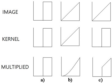
Now, when we have the original function as $y=x$ between 0 and 1 like a gray image, and assign a kernel function as the same as the original function, the convolutional integration is 1/3 in case (b). When we select another kernel function as 0 between 0 and 0.5, and 1 between 0.5 and 1, convolutional sum is 3/8 in case (c), which is slightly larger than case (b). The convolving function, or kernel function with exactly the same shape as original function does not produce the maximum value, or an extreme value. The resembling kernel function simply tends to produce relatively large convolutional integration. If we want to find the optimum kernel function with an upper limit integration value to produce the largest convolutional integration, the kernel found will be a delta function positioned at the largest independent variable place. If we call convolution as multiplication of coefficients and input pixel numbers, this operation could be called as linear with respect to the input pixel number which is regarded as independent variable. This example implies that application of the linear convolution may not be the unique way for classification of gray images.

It is considered that a nonlinear kernel could overcome the gray-direction-dependent solutions, either by resembling the nonlinearity of the visual reception operations in nature, or by taking rational reasoning for more efficient mathematical convergence.

2. Proposing kernel with square of subtraction

Ideal kernel should account for the similarity between images; images used for training and the images to be examined. We propose a kernel, the coefficient of which are directly subtracted from the local number of the pixel in common two-dimensional input image patches. Let’s consider a typical neural network architecture with one convolution layer with the new kernal and a pooling layer, see Fig. 2. We call it “Subtraction Neural Network” (SNN) afterwards.

An important attribute to use the feature map with the fully connected layer is that a better kernel coefficients should lead to larger feature map element, so that the weights applied to the feature map elements play a positive role to produce larger output. Therefore, we propose a kernel that the subtraction of between the input pixel number and the kernel coefficient is squared, its sign is reversed, and a bias is added. The feature map elements $X2$ are computed from the following Eq. (1):

where $X2$ is the feature map, $FX1$ is the transferred input two-dimensional image pixel number matrix by a linear function, $SF$ is the kernel coefficient matrix for subtraction, $BF$ is the bias of each kernel, $KF$ is the kernel serial index, $IF2$, $JF2$ are matrix element indices of a two-dimensional kernel, $I{1}^{*}$, $J{1}^{*}$ are two-dimensional matrix element indices of the input image pixel number matrix to match a moving kernel. It resembles the least square method, but with a negative sign here. Eq. (1) is quadratic, and thus nonlinear to both $FX1$ and $SF$.

Fig. 2SNN architecture to be considered: X1 – input image pixel matrix; FX1 – transferred X1 by linear function; SF – subtraction kernel coefficient matrix; BF – bias of subtraction kernel; X2 – feature map; FX2 – transferred X2 with sigmoid function; X3 – feature map after pooling; FX3 – transferred X3 by linear function; W4 – weights between fully connected layer and the output layer; B4 – bias between the fully connected layer and the output; X4 – output before activation function; FX4 – output after sigmoid activation function

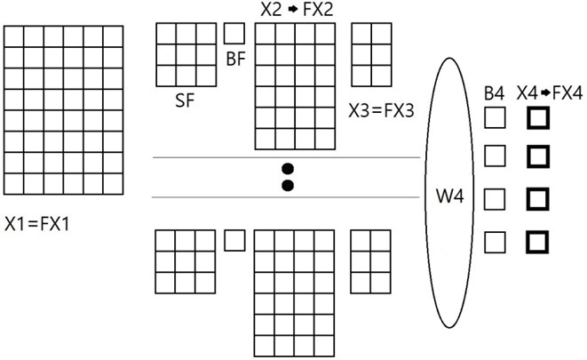
A pooling layer with arbitrary size of pooling filter often follows the above convolution layer, and the present architecture has one. Training of the subtracting kernel coefficients requires partial derivatives of the total error E_t with respect to each kernel coefficient $SF$ and kernel bias $BF$, that is:

The partial derivative of the total error in Eq. (2) is obtained from Eq. (1), and the derivative of $X2$ over the kernel coefficient $SF$ includes the kernel coefficient $SF$ itself as well as the $FX1$, that is:

It would be meaningful to compare the present proposal of nonlinear form of SNN with an existing common linear convolutional neural network. We consider a linear CNN with the same architecture as that of the above proposed nonlinear SNN of Fig. 2 except the kernel part, see Fig. 3.

Fig. 3CNN architecture to be compared: CF means linear convolutional kernel: X1 – input image pixel matrix; FX1 – transferred X1 by linear function; CF – linear convolution kernel coefficient matrix; BF – bias of linear kernel; X2 – feature map; FX2 – transferred X2 with sigmoid function; X3 – feature map after pooling; FX3 – transferred X3 by linear function; W4 – weights between fully connected layer and the output layer; B4 – bias between the fully connected layer and the output; X4 – output before activation function; FX4 – output after sigmoid activation function

When we use an existing linear convolutional kernel in the convolutional neural network, the feature map elements are computed from convolution between the kernel elements and the input image pixel number matrix elements as follows:

The derivatives of $X2$ with respect to CF for the convolutional kernel are also different from Eq. (4) for the subtraction kernel, that is:

Eq. (4) of the nonlinear subtraction kernal contains the same variable FX1 as Eq. (6) but twice larger. Another difference between the new subtraction kernel and the conventional linear convolutional kernel is that Eq. (4) involves SF term itself like an independent variable, which represent inherent nonlinearity of the present subtraction kernel. It is expected that the training time for a SNN should be similar to that of the corresponding linear CNN with the same architecture, if the number of epoch iteration is retained. If convergence criteria is limiting the total error allowance, training time becomes dependent on the performance of a network. Comparison is needed to examine the training efficiency of the two networks, nonlinear and linear ones.

3. Application of the present nonlinear subtraction approach

The nonlinear subtraction kernel approach proposed here is examined against two sets of images: 4 black and white images, and 4 gray images.

3.1. Black and white images

Four simple geometries are chosen as a classification problem. All four shapes are symmetric with respect to vertical line. Their widths and heights are the same, their positions are the same, and are at centers of the whole images. Pixel matrices of all four input images have size of 100×100.

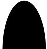
Fig. 4Four black and white images used for comparison of present nonlinear SNN and existing linear convolutional neural network: a) square, b) parabolic on both sides, c) half-elliptic; d) trapezoidal

a)

b)

c)

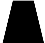
d)

Number of kernels is chosen as 4, kernel size is 3×3, and filter size of pooling is 1×1 which is the same as no pooling as default. Zero padding is not used during computation process from the input matrix to the feature map. Learning rate of 0.0005 is used.

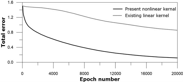
Training of the SNN shows decrease of the total error as training number increases, see Fig. 5.

The training of the present nonlinear subtraction kernel shows faster decrease of the total error than the existing linear kernel as the iteration number continues. This is a clear indication that the present nonlinear kernel performs better than the existing linear kernel for the given image data sets, taking account that both networks have the same network architecture.

Trained SNN can be examined to any new image. Image (a) of Fig. 4 is chosen for checking the ability to distinguish the four original figures of Fig. 4 as self-assessment. Because the image was the given information for training of the SNN, the ideal expectation of the application of Fig. 4(a) is close to 1.0. The application results depend on the iteration number, and the accuracy increases as the iteration number increases, see Fig. 6.

Fig. 5Total error versus iteration number for black and white images: real line – present nonlinear kernel; dotted line – existing linear kernel

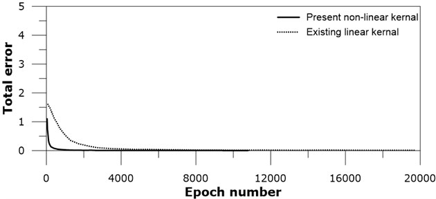
Fig. 6Output of application of image Fig. 4(a): real line – present nonlinear kernel; dotted line – existing linear kernel

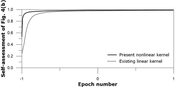
Both existing linear and present nonlinear kernel networks produce asymptotic approach toward 1.0 after many training iterations. The present nonlinear kernel network approaches 1.0 earlier than the existing linear kernel network. This difference also demonstrates the effectiveness of the present nonlinear kernel. Other self-assessments on Figs. 4(b, c, and d) show similar trends to Fig. 4(a).

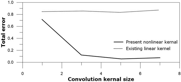
Optimum kernel size has attracted interest to many neural network modelers. The optimum kernel size may be dependent to many relevant factors like image pattern, existence of background, or color style, and their relationship has not yet been clearly arranged. Although the number of black and white images is not large, it would be meaningful to see the effect of the kernel size by applying neural networks to these images. Pooling process is not included in these tests, in other words, 1×1 pooling is applied to these tests. Tested kernel sizes are all square, i.e. 1×1, 3×3, 5×5, and 7×7. The total errors after 20000 training epoch iterations for several kernel sizes of the present nonlinear SNN and the existing linear neural network are shown in Fig. 7.

3×3 kernels exhibited relatively best results for both the present nonlinear SNN and the existing linear neural network compared to other sized kernels. Optimum kernel size may depend on various parameters like pattern type, micro-pattern frequency, or image edge shape, and is not further investigated here. Important thing is that 3×3 kernels for the present nonlinear neural network is better than that of the linear neural network work, and all other sized kernels have the same trend.

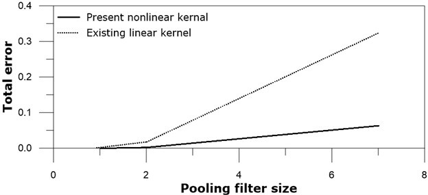
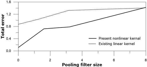
Pooling is another nonlinear process, and often adopted after convolution process. Tests on the max-pooling filter size are carried out to see their effect. Retaining 3×3 kernel size, square pooling filter sizes of 1×1 (means no pooling), 2×2, and 7×7 are examined after both the present nonlinear subtraction kernel convolution and the existing linear kernel convolution, see Fig. 8.

No pooling case produces the smallest total error after 20000 training iterations for both the present nonlinear kernel network and the existing linear kernel network. 2×2 pooling filter shows the next best results to no pooling. This result may be related to the images of Fig. 4, and could be thought as specific result, rather than general one. All pooling filter sizes of the subtraction nonlinear kernel network are better than the existing linear kernel network. The present examination results on the pooling filter sizes are based on limited number of images, and finding optimum pooling filter size for other images may vary.

Fig. 7Total error versus kernel size: real line – present nonlinear kernel; dotted line – existing linear kernel

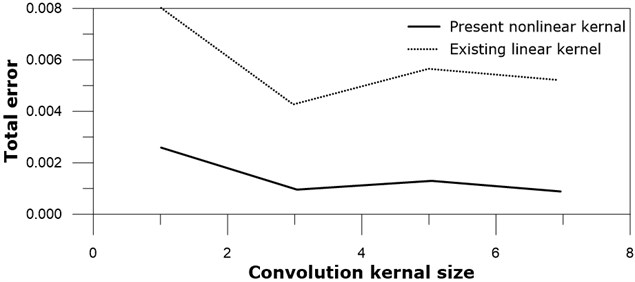
Fig. 8Total error versus pooling size: real line – present nonlinear kernel; dotted line – existing linear kernel

3.2. Gray images

Gray images have different characteristics from black and white images from mathematical point of view. Gray image pixel is expressed as an intermediate real number between 0 and 1 or their multiples, respectively, while black and white image pixel is expressed by bimodal manner like binary numbers. Behavior of convolution kernel in the CNN may depend on image type.

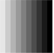
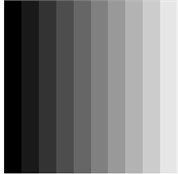
Selected gray images are all square in shape filled with vertical gray stripes, see Fig. 9. As the first step to examine the present nonlinear kernel, it would be meaningful to test simple patterns. Vertical stripes mean that they are virtually one-dimensional, and examination results are expected to provide intuitive results. Background color is white. Image sizes are 20×20, while the sizes of gray parts are all 10×10.

Fig. 9(a) image is vertical stripes getting darker in the right side, Fig. 9(b) image is the horizontally reversed image of Fig. 9(a), Fig. 9(c) is plain gray of 50 % black, and Fig. 9(d) is combination of two wide vertical gray stripes of 20 % and 80 % black.

Number of kernels chosen for tests is 4, kernel size is 3×3, and pooling filter size is 1×1 (no pooling). Zero padding is not used during computation process from the input matrix to the feature map. Learning rate of 0.0005 is used.

The total errors during training procedure decrease as the epoch iteration number increases, see Fig. 10. The training accelerate optimization of convolution kernel coefficients effectively for the present nonlinear kernel neural network, while it seems that the speed of training existing linear kernel network is not high. Considering the fact that the same neural network architecture is for both networks, this result may support the usefulness of the present nonlinear kernel, although the present test results are based on only four specific gray images.

Trained nonlinear subtraction kernel CNN can be examined to any new image. Image of Fig. 9(a) is chosen for checking the ability to distinguish the four original figures of Fig. 9 as self-assessment. Because the image was the given information for training of the subtraction kernel neural network, the ideal expectation of the application of Fig. 9(a) is close to 1.0. The application results show that the accuracy increases with the epoch iteration number, and the outputs eventually converge to 1.0, see Fig. 11.

Fig. 9Four gray images to be examined with present SNN and CNN: a) darker right, b) darker left, c) half-gray; d) two gray tones, i.e. 20 % and 80 % black color

a)

b)

c)

d)

Fig. 10Total error versus iteration number: real line – present nonlinear kernel; dotted line – existing linear kernel

Both existing linear and present nonlinear kernel networks produce asymptotic approach toward 1.0 after many training iteration. The present nonlinear kernel network approaches 1.0 earlier than the existing linear kernel network. This difference also demonstrates the effectiveness of the present nonlinear kernel. Other self-assessments on Figs. 9(b), (c), and (d) show similar trends to Fig. 9(a).

We look at the effect of the kernel size for the present nonlinear kernel and the existing linear kernel on the four test gray images. It would still be meaningful to see the effect of the kernel size by applying neural networks on our limited number of gray images. Pooling process is not included in these tests, in other words, 1×1 pooling is applied to these tests. Tested kernel sizes are all square, i.e. 1×1, 3×3, 5×5, and 7×7. The total errors after 20000 training epoch iterations of the present nonlinear SNN and the existing linear neural network are shown in Fig. 12.

5×5 kernel exhibits best results, and 3×3 kernel is the next for the present nonlinear subtraction kernel convolutional neural networks. On the other hand kernel size does not give much different total error for the existing linear kernel convolutional neural network. Optimum kernel size may depend on various parameters like pattern type, micro-pattern frequency, or image edge shape, and thus the present results could not be generalized for other images. It should be noted that 5×5 and 3×3 kernels for the present nonlinear neural network is better than that of the linear neural network work. The results may imply that overall behavior of the present nonlinear kernel convolution is promising compared to the existing linear kernel convolution.

Fig. 11Output of application of image Fig. 9(a): real line – present nonlinear kernel; dotted line – existing linear kernel

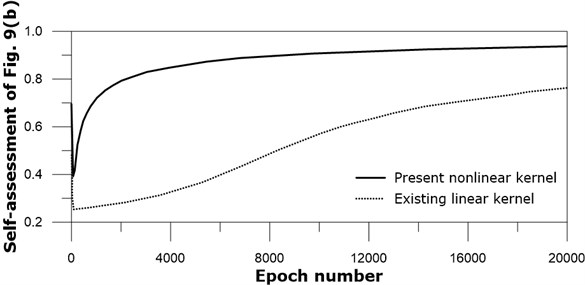
Fig. 12Total error versus kernel size: real line – present nonlinear kernel; dotted line – existing linear kernel

Pooling is another nonlinear process, and often adopted after convolution process. Tests on the max-pooling filter size are carried out to see their effects on the total error. Square pooling filter sizes of 1×1 (means no pooling), 2×2, 3×3, and 6×6 are examined after both the present nonlinear subtraction kernel convolution and the existing linear kernel convolution, while the convolution kernel size is kept 3×3, see Fig. 13.

1×1 pooling case, in other words, no pooling case produced the smallest total error after 20000 training iterations for both the present nonlinear kernel network and the existing linear kernel network. 2×2 pooling filter shows the next best results to no pooling. It should be noted that this result is obtained from the four images of Fig. 9, and could be thought as specific problem, rather than general one. 3×3 pooling filter sizes of the subtraction nonlinear kernel network are better than the existing linear kernel network. The total errors of 6×6 pooling filter networks for both the nonlinear kernel and the existing linear kernel show slow decrease, meaning poor performance. At least this large pooling filter size like 6×6 is not desirable for given gray images.

Fig. 13Total error versus pooling size: real line – present nonlinear kernel; dotted line – existing linear kernel

4. Conclusions

The concept of finding a linear kernel which results in the largest integration for given black and white image matches well with the existing linear kernel convolutional neural network, but not for gray images. A kernel composed of a bias and negative summation of square of subtraction between the input pixel number and the kernel coefficient itself within the moving input pixel patch for convolution is proposed here. The square of subtraction represent the intensity of similarity between the kernel coefficient matrix elements and the image pixel number matrix elements as expressed in the summation equation. It resembles the least square method, but with a negative sign here and biases are added. Training of the neural network to obtain optimum kernel coefficients requires a derivative with respect to the kernel coefficient includes the input pixel number and the kernel coefficient itself, and makes the formation nonlinear.

The present nonlinear kernel formulation is examined to two sets of images: four black and white images, and four gray images. The network training results are compared to those of corresponding CNN with the same architecture and parameters except the kernel. Application results show that the present nonlinear subtraction kernel is more efficient than the existing linear convolutional kernel, although the tests are limited to two sets of images: black and white images and gray images. After all, the nonlinear kernal of the present network produced fast decrease of the total error, and its intention is well explained in the kernal equation.

It is believed that the present nonlinear kernal is based on sounder background to obtain maximum outputs. Further examinations against various images and conditions are needed to enhance reliability of the presently proposed nonlinear subtraction convolution kernel of the convolutional neural network. It seems that application areas of the present nonlinear subtraction kernel CNN could be expanded to full color images as well.