Abstract
Three sediment transport formulas by Lund-CIRP (2012), van Rijn (1998), and Soulsby (1997) were applied for this study with field data by Yoon (2008) and several sedimentary variables of Nakdong Estuary in a coupled numerical modeling system, CMS. CMS is adopted to compare the measured depth change data and the calculated depth change data. As a result, the Lund-CIRP formula with mean grain size (0.25 mm) and multi-bottom friction coefficients based on the mean grain size distribution had higher accuracy (1.6 %) than the other formulas. The Soulsby formula has higher accuracy for multi-grain size and 0.06 of bottom friction coefficients. The van Rijn formula has high accuracy at shallow water areas such as a river. In this study, it is judged that the accuracy of the van Rijn cases was low because the water depth of the Nakdong Estuary and the nearby sea area rapidly deepens.
1. Introduction
Numerical modeling will be used to analyze flow patterns to make predictions for morphological change by the construction of coastal structures. The past studies were considered only the effect of a single factor to understand morphological transformation in Nakdong Estuary (Park et al, 2009) [1]. But results from past researches were not insufficient to prove the relationship between the effects of each different factors. To investigate the effects of factors, an appropriate numerical model scheme was needed. Bed elevation changes of Nakdong River by HEC-RAS (Kim and Kim, 2020) [2], behavior analysis of salt water by EFDC (Kim, 2019) [3], and settlement in the soft ground by K-Embank and Soil Works (Park and Ryu, 2019) [4] were representative researches to analyze the characteristic of Nakdong Estuary area.
Most numerical models have similar flow equations; however, wave equations and sediment transport equations differ and result in different output. Therefore, the wave equation and sediment transport equations must be investigated to determine which numerical model is proper for particular study area.
Many researchers have coupled flow, wave, and sediment models to make better predictions. John et al. (2008) [5] coupled SWAN (Simulating Waves Nearshore) for wave (coupled by MCT (Model Coupling Toolkit) and ROMS (Regional Oceanographic Modeling System) for flow, and used flux formulation for sediment (advection-diffusion equation for suspended sediment transport and Soulsby’s formula for bedload transport). This coupled model worked well for wave and flow, but part of sediment concentration was not accurate. SWAN and SHORECIRC (SHORE CIRCulation) were coupled by Tang et al. (2009) [6]. This model used the convection-diffusion equation for sediment transport. When this model was tested, problems such as restriction on time step and high-resolution flow scheme for the coupled system were found. These examples demonstrate why model coupling is complicated and why it is needed to more accurately determine morphological transformations in a given study area.
Some popular package tools include: Delft-3D, ECOMSED (Estuarine, Coastal and Ocean Model system with SEDiment), EFDC (Environment Fluid Dynamic Code), and SMS (Surface water Modeling System). These programs include powerful tools for calculating wave, flow and sediment transport. Many programs are based on 3D coordinate systems and 3D formulas. Especially, the wave-induced current field at the time is quantitatively described by using a numerical modeling system CST3D which adopts rearrangement of driving wave-induced forces, and the PESM for computation of advection terms by Kim et al. (2014) [7, 8].
Many 3D models still have problems with complicated topography and suspended sediment transport at the shallow area. For the Nakdong Estuary, 2D depth-integrated models are sufficient for this shallow water body and calculation period because vertical water flow values are not widely variable.
This paper aims to predict the long-term effects of sediment movement in the Nakdong Estuary, and to evaluate which the formula is most suitable for the Nakdong Estuary among existing excellent sediment transport formulas.
2. Characteristics analysis in the study area
The pattern of the tide in the study area is semi-diurnal tide. Tidal constituents from water surface elevation data were processed by T-Tide (harmonic analysis program; Pawlowicz, 2002) [9]. According to coastal morphology classification, the study area with a tidal range of 0 to 1 m is classified as microtidal Estuary (tide range in 0 to 2 m). Characteristics of barrier islands in microtidal condition are narrow and linear barriers, and inlets migrate if the environment around the islands is not stabilized. Barrier islands can be overwashed by storms. The sources of creation and development from river and littoral flow into a shoal of barrier islands. The barrier islands in the Nakdong River have all these microtidal characteristics.
Fig. 1KHOA (Korea Hydrographic and Oceanographic Agency) and KMA (Korea Meteorological Administration) stations located around the Nakdong Estuary, the Republic of Korea
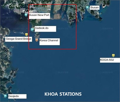
To understand the mechanism of water flow in the research area, the wind force is an important source to generate waves on water surface. Hourly wind data were obtained for Gadeok-do station from 1993 to 2013 (Location in Fig. 1).
Another important oceanographic variable is wave action. Hourly mean wave data between 2007 and 2013 was obtained from the KMA wave buoy installed at southeast Geoje-do (Fig. 2).
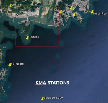
Waves from the southwest of the Nakdong Estuary were dominant from 2007 to 2013. Waves from 0.5 to 1.0 m were mainly generated in the southwest of the study area (Fig. 3). The maximum wave height was 2.37 m on November, 11th, 2009. The season, June to September had the highest potential for typhoons and associated wave heights over 1.0 m. Typhoons are the main event to transform shoreline and littoral with strong wind, heavy rainfalls, and higher river discharges.
Typhoons typically originate from the southwest of the Nakdong Estuary. Typhoons directly impacted the study area in 1991 (GLADYS), 1998 (YANNI), 2002 (RUSA), 2003 (MAEMI), and 2007 (NARI) in this research period. The highest instantaneous wave heights were 17 m during MAEMI in 2003.
Incoming freshwater discharge from the Nakdong River was measured at the entrance of the Nakdong Estuary. Gupo station controlled by K-water is the closest station to report water surface elevation. Data is available for daily water surface elevation from 1982 to 2013. Water surface elevation around the entrance of the Nakdong River is affected by river flow, inflow from the branch, rainfall, and tide. Gupo station is the only station with accurate data to know the total amount of inflow on the Nakdong Estuary (Fig. 4).
Fig. 2A wave rose based on Geoje Buoy data (from 2007 to 2013) and the buoy is located 33.5 km from the Nakdong Estuary, the Republic of Korea
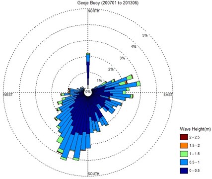
Fig. 3Daily mean wave height at Geoje-do buoy from 2007 to 2013, located 30 km from the south of Nakdong Estuary, the Republic of Korea
From the trend line, water surface elevation had increased from 1983 to 1988, and was stable to 2009. But, after 2009, water surface elevation is up to 1 m in the trend line. The red line in Fig. 4 assigned the time of the completed construction of the Nakdong Estuary Dam. The rise of the water surface appeared to be due to the Nakdong Estuary Dam and Busan New ports. Daily oscillations were detected due to the tide effect near the Nakdong Estuary. The tide is dominant in the study area.
After the construction of the Nakdong Estuary Dam, discharges from the dam may have influenced morphological transformations in the area. The Nakdong Estuary Dam has been keeping a schedule of discharge based on the amount of inflow from the upper reaches of the Nakdong River. The Nakdong Estuary Dam had an enormous discharge rate (up to 1,600×106 m3/day) in the summer season between 1996 and 2006 (Fig. 5).
Fig. 4Water surface elevation at Gupo station, upside of the Nakdong Estuary Dam, during 1982 to 2013 with 10th order polynomial trend line
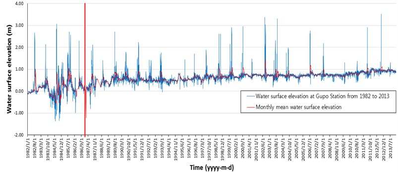
Fig. 5Discharge rate from the Nakdong Estuary Dam, located between Eulsuk-do and Busan, the Republic of Korea between 1996 to 2006 (Yoon, 2008) [11]
![Discharge rate from the Nakdong Estuary Dam, located between Eulsuk-do and Busan, the Republic of Korea between 1996 to 2006 (Yoon, 2008) [11]](https://static-01.extrica.com/articles/21919/21919-img6.jpg)
3. Numerical model conditions
The study area is shallow near barrier islands, and more time-consuming 3D numerical models are not necessary for analysis. Many 2-dimensional numerical models are designed to solve environmental material transport; however, CMS (Coastal Modeling System) in the SMS platform is more focused on sediment transport and shoreline change. Therefore, CMS may be the best numerical platform to study the transformation of barrier islands in the Nakdong Estuary system. CMS was developed and maintained by CIRP (Coastal Inlets Research Program) and Aquaveo. It has been used for studying the Sebastian Inlet system in Florida (Zarillo and Brehin, 2007) [10] with great success. The overall workflow of CMS is described in Fig. 6.
The CMS has two parts (CMS-Flow and CMS-Wave) that are coupled within SMS. CMS-Flow is a 2-dimensional depth-averaged nearshore circulation model. The hydrodynamic equations are the general depth-averaged continuity and momentum equations. CMS-Flow calculates currents and water levels, sediment transport, morphological change, and salinity. CMS-Wave is a phased-averaged model for the propagation of directional irregular waves over complicated bathymetry found nearshore. It solves the wave action balance equation by FDM (Finite Difference Method). This equation represents 2D variations in wave energy in space. For studying the detailed variation of sediment transport pattern of the Nakdong Estuary analysis of multi grain size distribution is required. In this study area, the bottom has multi grain size distribution (sand, fine-grain sediments, and mixtures of sand and fine grain sediments). Multi grain size is calculated by CMS. Interaction between tidal, wave, and sediment transport processes was calculated by steering module in CMS (Sanchez et al., 2012) [11].
Fig. 6CMS (Coastal Modeling System) flow chart (from CMS User’s Manual, Sanchez et al., 2012) [8]
![CMS (Coastal Modeling System) flow chart (from CMS User’s Manual, Sanchez et al., 2012) [8]](https://static-01.extrica.com/articles/21919/21919-img7.jpg)
CMS has multiple sediment transport formulas: Lund-CIRP (2012) [11], Soulsby (1997) [12], and van Rijn (1998) [13] that can be applied. Three sediment formulas by Lund-CIRP, van Rijn, and Soulsby were applied for this study area with field data by Yoon (2008) [14]. According to the characteristics of each formula, different transport formulas may produce different patterns of morphology change in the study area. After modeling using these three formulas and data from 1982 and 1986 nautical charts, the most reliable formula will be identified and used to model the long-term morphological transformation of barrier islands in the Nakdong Estuary.
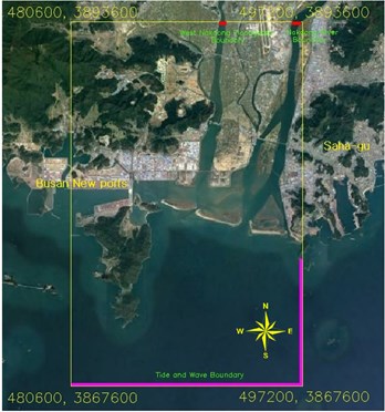
As shown in Fig. 7, Data for the numerical model was obtained from monitoring stations within the river and from offshore tide and wave buoys. The origin of the model grid is E 480,600 m and N 3,867,600 m (UTM units). The model area has a width of 16,600 m (east to west) and a length of 26,000 m (north to south). Each rectangular grid cell is 100 m by 100 m (166 × 260 grids).
Initial conditions, used to establish the numerical model grid including water depth and shoreline position, were extracted from nautical charts. Bathymetric data were extracted from Electronic Nautical Charts (ENC) or digitalized files from scanned charts using AUTOCAD if ENC were unavailable. The initial grain size distribution was obtained from Kim and Ha (2001) [15] and applied to the input grid. Boundary conditions were classified as either offshore boundary conditions or a land boundary conditions that affect ocean dynamics and sediment transport. Wave boundary conditions were daily significant wave data calculated from hourly observations at the Geojae buoy with data available beginning in 1998. Tide data was obtained from two weather stations located at Busan New ports and Gadeok-do. Tidal data was processed by the harmonic analysis function in T-Tide applied to CMS. Tidal variations will be calculated using the M2 (principal lunar semidiurnal), S2 (principal solar semidiurnal), K1 (lunisolar diurnal), and O1 (principal lunar diurnal) variations. Hourly wind data collected at Gadeok station were also applied to increase the accuracy of the model. Lateral boundary inputs to the model utilize daily flow rates for the West Nakdong floodgates and daily water surface elevation data from Gupo station located at the upper Nakdong Estuary Dam. These boundary values from measured data will ensure the reliability and accuracy of the numerical model analysis and prediction of morphological transformation for the Nakdong Estuary.
Fig. 7Model grid area (horizontal distance: 16.6 km, vertical distance: 26.0 km) and boundary condition section (pink line)
To assess the accuracy of topographic calculations of the model, it is necessary to compare the bathymetric data throughout the study area between 1982 and 1986 (Fig. 8 and 9).
Fig. 8Measured morphological change (red means depositions and blue means erosions) around barrier islands, located the Nakdong Estuary, the Republic of Korea between 1982 and 1986
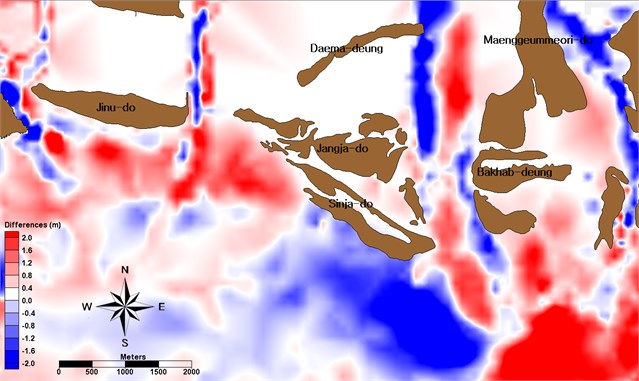
Jinu-do had erosion at the south shoreline and the channel between Gadeok-do and Jinu-do (Fig. 8). Deposition occurred at the southwest of Shinja-do while erosion happened at the southeast shoreline. The channel between Shinja-do and Bakhab-deung had morphological transformation within 2 m, and deposition occurred at east and southeast of Bakhab-deung due to the dredging for construction of the Nakdong Estuary Dam and creating the industrial complex at Myeongji-dong. The overall pattern of morphological change around barrier islands shows a pattern of the normal distribution with a relatively small variation (Fig. 9).
The numerical model simulations to compare with the frequency distribution of depth changes need detailed boundary conditions to achieve accurate results. The list of boundary conditions that produce force in the model is in Table 1.
Fig. 9Frequency distribution of depth change, located the Nakdong Estuary, the Republic of Korea from 1982 to 1986
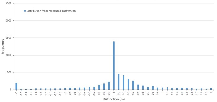
Table 1List of tidal constituent boundary conditions to perform CMS-Flow and CMS-Wave
Tide | Tidal constituents | Amplitude (m) | Phase (degree) |
M2 | 0.544 | 240.5 | |
S2 | 0.257 | 267.8 | |
K1 | 0.078 | 155.9 | |
O1 | 0.043 | 133.1 | |
River | River name | Station | Input type |
West Nakdong River | Noksan floodgates | Daily average flow rate (m3/s) | |
Nakdong River | Gupo | Daily average water surface elevation (m) | |
Wave | Station | Input type | |
Geoje buoy | Daily average (height, period, direction) | ||
Wind | Station | Input type | |
Gadeok-do station | Hourly average(speed, direction) | ||
Table 2List of cases to calibrate the model
Case | Comparison |
1 | Spatially multi grain size with Lund-CIRP, Soulsby, and van Rijn formulas |
2 | Spatially mean grain size (0.25 mm) with Lund-CIRP, Soulsby, and van Rijn formulas |
3 | Changing grain size, including separate model runs for 0.2 mm, 0.25 mm, 0.3 mm, and 0.35 mm with Lund-CIRP formula |
4 | mean grain size (0.25 mm) with multi-bottom friction coefficients with Lund-CIRP formula |
Boundary conditions were applied in the model grid and CMS control panel. Model simulation time and matrices solver was chosen in the control panel of CMS-Flow and Wave. To calibrate the model, simulation time was entered from January 1st 1982 to January 1st 1987, and applied matrices solver was Gauss-Seidel, CMS-Flow and CMS-Wave are coupled through a steering option that sends water levels and flows to the CMS-Wave grid and wave forcing to the CMS-Flow grid. Sediment equations and initial grain size distribution were chosen in the sediment tab in the CMS-Flow control panel. The cases to calibrate the numerical model were performed based on the conditions listed in Table 2.
4. Comparison of measured and calculated morphological change
Case 1 calculations were based on multi-grain size distribution on the study area (Kim and Ha, 2001). Within Case 1 the model results using the Lund-CIRP and van Rijn sediment transport formulas produced accurate sediment transport pattern with measured data around Jinu-do and west of Shinja-do compared with model results based on the Soulsby formula. Soulsby sediment transport formula produced deposition between Jinu-do and Gadeok-do (Fig. 10).
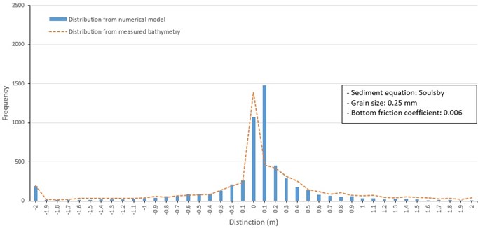
Frequency distributions of depth changes produced by the three sediment transport formulas included a model depth change of +0.1 m and a secondary model change of 0 m (Fig. 10, 11, and 12). This differs from the depth change distribution from measured data shown in Fig. 8, which has a distinctive frequency peak at 0m. However, the overall shape of the distribution from predicted and measured data are similar, including a secondary frequency peak of depth change at –2 m. Despite the limitations of the measured data to drive and calibrate the model and the difficulty of predicting sand transport, the overall results show the patterns of sediment transport around Jinu-do and Shinja-do varied in the range of measured data.
Fig. 10Frequency distribution of depth change around barrier islands from 1982 to 1986 (Lund-CIRP, multi grain size)
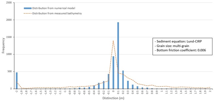
Fig. 11Frequency distribution of depth change around barrier islands from 1982 to 1986 (Soulsby, multi grain size)
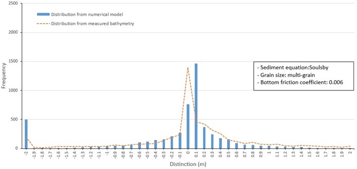
Fig. 12Frequency distribution of depth change around barrier islands from 1982 to 1986 (van Rijn, multi grain size)
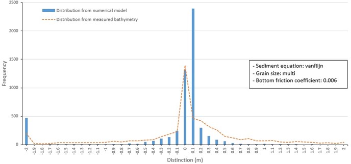
Fig. 13Frequency distribution of depth change around barrier islands from 1982 to 1986 (Lund-CIRP, 0.25 mm mean grain size)
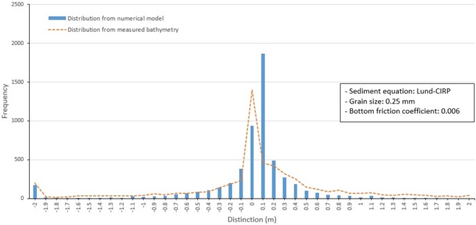
Fig. 14Frequency distribution of depth change around barrier islands from 1982 to 1986 (Soulsby, 0.25 mm mean grain size)
Case 2 runs to address the effect of applying a spatially uniform distribution mean grain size (Kim and Ha, 2001) to three sediment transport formulas (Fig. 13 to 15). The results based on the uniform mean grain size is similar to the spatially varying mean grain. The calculated frequency distributions of model depth change based on the Lund-CIRP and Soulsby sediment transport formulas were similar to those of Case 1 and overall similar to depth changes between 1982 and 1986 (Fig. 13 and 14). Results calculated by van Rijn formula included a notable higher frequency of depth change of 0.1 m compared to results from the other sediment transport formulations (Fig. 15).
Fig. 15Frequency distribution of depth change around barrier islands from 1982 to 1986 (van Rijn, 0.25 mm mean grain size)
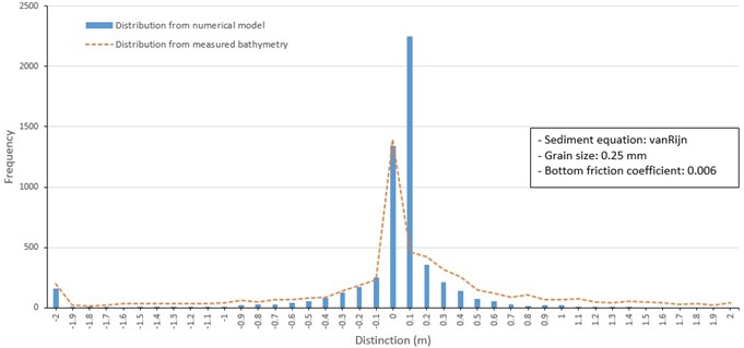
Fig. 16Frequency distribution of depth change around barrier islands from 1982 to 1986 (Lund-CIRP, 0.2 mm grain size)
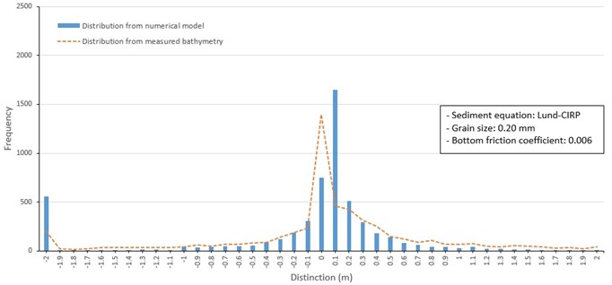
Fig. 17Frequency distribution of depth change around barrier islands from 1982 to 1986 (Lund-CIRP, 0.3 mm grain size)
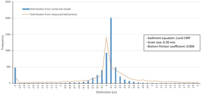
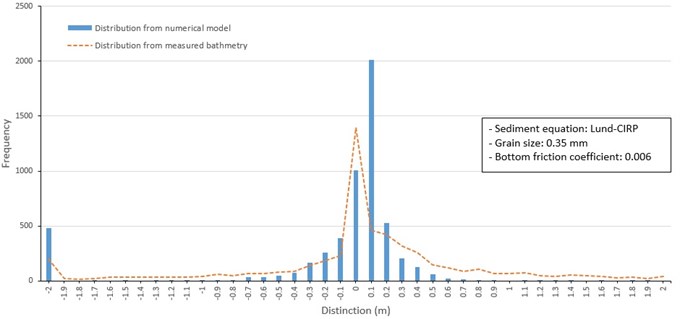
Case 3 examines the influence of changing mean grain size on model performance. Thus, three separate model runs were conducted using a uniform grain size over the model grid including 0.2 mm. 0.3 mm, and 0.35 mm (Fig. 16 to 18). The model test applying 0.2 mm mean grain size uniformly distributed over the model grid (Fig. 16) overestimated erosion and deposition around shorelines of barrier islands. Erosion and depth increase of up to 4 m occurred in channels between Jinu-do and Shinja-do and between Shinja-do and Bakhab-deung. It also made deposition within 4 to 5 m at offshore of barrier islands and exit of the Nakdong River. The model test case of applying 0.3 mm grain size uniformly over the model grid (Fig. 17) provided similar results to those from the 0.2 mm size in Fig. 14. However, erosion and deposition values were underestimated around the shoreline of Jinu-do and Shinja-do. In the case of 0.35 mm mean grain size applied over the grid (Fig. 18), reduced the movement of sand and consequently reduced the magnitude of depth changes compared to the results of model tests of other particle sizes.
Fig. 18Frequency distribution of depth change around barrier islands from 1982 to 1986 (Lund-CIRP, 0.35 mm grain size)
Based on the model results from applying different sediment grain size values over the model grid, 0.25 mm was considered the appropriate mean grain size for model tests involving a uniform the mean grain size in the study area.
Fig. 19Computed morphological change (red is deposition, and blue is erosion) around barrier islands between 1982 and 1986 (Lund-CIRP, mean grain size: 0.25 mm, and multi bottom friction coefficients based on multi grain size distribution)
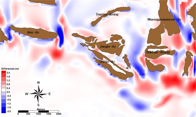
In Case 4, a spatially uniform mean grain size was combined with spatially varying friction coefficients to account for variations in topography and smooth that affect flow speeds (Fig. 19 and 20). In the measured data sets, apparent erosion was present within the waterway near west and east Bakhab-deung. This was due to the dredging of the waterway. Consequently, model results shown in in Fig. 19 and 20, did not include dredging by the construction of the Nakdong Estuary Dam and creating the Myeongji complex.
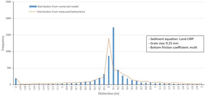
Fig. 20Frequency distribution of depth change around barrier islands from 1982 to 1986 (Lund-CIRP, mean grain size: 0.25 mm, multi bottom friction coefficients based on multi grain size distribution)
5. Conclusions
The numerical model was able to calculate the sediment transport with enough accuracy to produce topographic changes similar to measured changes to a first order. Further, the similarity of the calculated and measured frequency distribution of depth changes over long-time scales indicated that sediment transport calculations were realistic and not over-calculated.
Table 3Error rates between measured depth change and computed depth changes (calculated by Normalized Root Mean Squared Error)
Case Name | Error rate (%) |
Spatially multi grain size with Lund-CIRP formula: bottom friction coefficients = 0.006 | 2.27 |
Spatially multi grain size with Soulsby formula: bottom friction coefficients = 0.006 | 2.15 |
Spatially multi grain size with van Rijn formula: bottom friction coefficients = 0.006 | 2.33 |
Spatially mean grain size (0.25 mm) with Lund-CIRP formula: bottom friction coefficients = 0.006 | 2.26 |
Spatially mean grain size (0.25 mm) with Soulsby formula: bottom friction coefficients = 0.006 | 2.34 |
Spatially mean grain size (0.25 mm) with van Rijn formula: bottom friction coefficients = 0.006 | 2.34 |
Spatially uniform grain size (0.20 mm) with Lund-CIRP formula: bottom friction coefficients = 0.006 | 2.48 |
Spatially uniform grain size (0.30 mm) with Lund-CIRP formula: bottom friction coefficients = 0.006 | 2.58 |
Spatially uniform grain size (0.35 mm) with Lund-CIRP formula: bottom friction coefficients = 0.006 | 2.56 |
Spatially mean grain size (0.25 mm) with Lund-CIRP formula: multi-bottom friction coefficients | 1.60 |
The evaluation for the accuracy of depth change was confirmed by the applied grid area (5544 grids) without land-cells The Normalized Root Mean Squared Error (RMSE) was used to evaluate the accuracy of results by comparing differences between measured depth changes and computed depth changes.
As shown in Table 3, the Lund-CIRP formula with mean grain size (0.25 mm) and multi-bottom friction coefficients based on the mean grain size distribution had higher accuracy (1.6 %) than other cases. The Soulsby formula has higher accuracy for multi grain size and 0.06 of bottom friction coefficients. We usually know that the van Rijn formula has high accuracy in shallow water areas such as a river. In this study, it is judged that the accuracy of the van Rijn cases were low because the water depth of the Nakdong Estuary and the nearby sea area rapidly deepens. The CMS numerical model with the Lund-CIRP sediment transport formula as presented will provide valuable information to minimize negative effects on the morphology of barrier islands and to maintain the open waterways properly. Also, the CMS numerical model can be used to accurately assess possible environmental and morphological impacts in the Nakdong estuary. Thus, it is possible to perform a numerical model prediction to quantify the long-term influence of the construction of the Nakdong Estuary Dam.
References
-
Soon Park, Han-Sam Yoon, Hyo-Bong Park, Seung-Woo Ryu, and Cheong-Ro Ryu, “Analysis of wave distribution at Nakdong river estuary depending on the incident wave directions based on SWAN model simulation,” (in Korean), Journal of the Korean Society for Marine Environment and Energy, Vol. 12, No. 3, pp. 188–196, Jan. 2009.
-
S.-J. Kim and C.-S. Kim, “Analysis of bed changes of the Nakdong River with opening the weir gate,” (in Korean), Ecology and Resilient Infrastructure, Vol. 7, No. 4, pp. 353–365, Dec. 2020, https://doi.org/10.17820/eri.2020.7.4.353
-
T. Kim, “Study on the behavior analysis of salt water according to the operation of Nakdong river estuary barrage,” (in Korean), Ph.D. thesis, Inje University, 2019.
-
C.-S. Park and M.-Y. Ryu, “Characteristics of long-term settlement in the soft ground of Nakdong river by numerical analysis,” (in Korean), Journal of the Korean Geosynthetics Society, Vol. 18, No. 3, pp. 55–67, Sep. 2019, https://doi.org/10.12814/jkgss.2019.18.3.055
-
J. C. Warner, C. R. Sherwood, R. P. Signell, C. K. Harris, and H. G. Arango, “Development of a three-dimensional, regional, coupled wave, current, and sediment-transport model,” Computers and Geosciences, Vol. 34, No. 10, pp. 1284–1306, Oct. 2008, https://doi.org/10.1016/j.cageo.2008.02.012
-
H. S. Tang, T. R. Keen, and R. Khanbilvardi, “A model-coupling framework for nearshore waves, currents, sediment transport, and seabed morphology,” Communications in Nonlinear Science and Numerical Simulation, Vol. 14, No. 7, pp. 2935–2947, Jul. 2009, https://doi.org/10.1016/j.cnsns.2008.10.012
-
H. Kim, J. Ahn, C. Jang, J. Jin, and B. Jung, “Extension of piecewise exact solution method for two – and three-dimensional fluid flows,” Journal of Vibroengineering, Vol. 15, No. 3, pp. 1243–1254, Sep. 2013.
-
H. Kim, J. Y. Jin, D. H. Hwang, C. Jang, and H.-S. Ryu, “Simulation of wave-induced alongshore current during high waves at Haeundae beach, Korea,” Journal of Vibroengineering, Vol. 16, No. 8, pp. 3726–3739, Dec. 2014.
-
R. Pawlowicz, B. Beardsley, and S. Lentz, “Classical tidal harmonic analysis including error estimates in MATLAB using T_TIDE,” Computers and Geosciences, Vol. 28, No. 8, pp. 929–937, Oct. 2002, https://doi.org/10.1016/s0098-3004(02)00013-4
-
G. A. Zarillo and F. G. A. Brehin, “Hydrodynamic and morphologic modeling at Sebastian Inlet, FL,” in Sixth International Symposium on Coastal Engineering and Science of Coastal Sediment Process, pp. 1297–1310, May 2007, https://doi.org/10.1061/40926(239)100
-
A. Sanchez, L. Lin, T. Beck, Z. Demirbilek, M. Brown, and H. Li, Coastal Modeling System User Manual. CIRP, 2012.
-
R. Soulsby, Dynamics of Marine Sands. London: Thomas Telford, 1997.
-
L. van Rijn, Principles of Coastal Morphology. Netherlands: Aqua Publications, 1998.
-
E.-C. Yoon and J.-S. Lee, “Characteristics of seasonal variation to sedimentary environment at the estuary area of the Nakdong,” (in Korean), Journal of Korean Society of Coastal and Ocean Engineers, Vol. 20, No. 4, pp. 372–389, 2008.
-
S. Kim S. and J. Ha, “Sedimentary facies and environmental changes of the Nakdong River estuary and Adjacent Coastal area,” (in Korean), Korean Journal of Fisheries and Aquatic Sciences, pp. 268–278, 2001.
About this article

This work was supported by the Daejin University Research Grants in 2022.
