Abstract
In order to supply the required water for purposes such as irrigation, municipal and industrial consumptions, etc., human beings have always attempted to diverse water and construct large and small water intakes near the great rivers. Therefore, water diversion from the main path, water flow regime and the sediment transported by it change. This paper simulates the flow hydraulic in intake from the direct path of a rectangular channel and Navier-Stokes equations are solved by Finite-Volume Method (FVM) using the SSIIM2 software in which the flow velocity profiles near the surface of the water, the turbulent kinetic energy and hydrostatic pressure distribution in different sections of the main channels and intake at a constant discharge of 11 lit/sec, with the intake discharge ratio of 0.31, the inlet Froude number of 0.13 and various turbulence models were calculated in 3D mode and compared with the experimental results and there were a good agreement between the obtained values and the experimental results.
1. Introduction
Water diversion from its original path has always been performed for purposes such as irrigation, municipal and industrial consumptions, etc. Diverted flow into the intake has complex properties leading to separation zones in the main channel and the intake. In this area of flow, the fluid particles move around at a limited distance from the wall and in fact this part of the lateral channel does influence the flow discharge. In other words, the separation zone reduces the effective intake section. In case of high flow rate the suspended particles in the water cause great damages to the facilities such as the pump and turbine. Also, due to changes in the velocity distribution in the intake usually the sedimentation occurs at the intake inlet that leads to reduced intake efficiency, the entrance of coarse sediment into the network, increasing the costs of de-sedimentation process. Any action that leads to reduced secondary and vortex flow in the intake inlet will lead to reduced accumulation of sediment in the intake and reduced sediments entering the intake. Many studies have been conducted on the flow diversion at the straight direction by the previous researchers. The first of these studies belonged to Taylor (1994) [1]. He has presented a graphical solution based on trial and error by the experimental study of an open channel. He suggested that changes in water depth near the intake are considered about 2 % of the maximum depth for a wide range of discharge ratios and Froude numbers in a 90 degrees branch. Law and Reynolds (1966) [2] conducted an analytical experimental study on the main channel and the diversion of equal width and presented a relation for the discharge ratios and the Froude number before the intersection at this channel and the ratio of the width of the diversion channel to the main channel. Barkdoll et al. (1998) [3] compared the flow in an open channel with the width to depth ratio of ½ with a flow pipe with the width to depth ratio of ¼ and related the velocity variation near the water surface which was equal with 0.36 to the secondary flows in open channels. Ramamurthy et al. (2007) [4] conducted the experimental study on a T-Junction and an open channel with rectangular cross-section and used various tools at different sections. They also have developed a 3D numerical model to characterize the flow specifications and compared the velocity values obtained from the experimental results and observed a good agreement. Neary and Sotiropoulos (1996) [5], reproduced the 3D factors measured in lateral intake flows in the 3D flow study of a T shaped intersection. These two researchers used the finite volume method to solve the relations and examined the flow rate in this field and simulated the trend of sediment moment of the bed-load qualitatively. Issa and Oliveira (1994) [6], simulated the 3D turbulent flows for the T shaped geometries. They solved the averaged time Navier-Stokes equations by the Reynolds method in the 3D mode (RANS) by the k-ε standard model and wall functions. Pirzadeh (2007) [7] examined the flow hydraulics numerically using the fluent software. In this study using RSM and - turbulence models the three-dimensional assessment of flow velocity profiles was performed and there were a good agreement between the experimental values and the obtained results. The present study includes the numerical simulation of flow hydraulic in direct intake from a rectangular channel and straight walls which is performed by SSIIM2 soft ware. The modeling is based on the experimental study of Barkdoll et al. (1998) [3] in which the flow velocity profiles near the surface of the water, the turbulent kinetic energy and hydrostatic pressure distribution in different sections of the main channels and intake were calculated to compare the existing turbulent models and were compared with the mentioned experimental results [3].
2. The characteristics of the experimental model
In the experimental study of Barkdoll et al. (1988) [3] the length of the main channel is 2.74 m and the intake channel is 1.68 m located at 90 degrees. The input discharge is 0.011 cubic meters per second, the depth is 0.31 m and the width of both channels is 0.152 m. Fig. 1 and Table 1 show schematic of the channel and the hydraulic characteristics of the flow, respectively [3].
Fig. 1The geometric characteristics of the flume
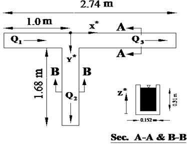
Table 1Hydraulic characteristics of flow
Froude number | Reynolds number | Intake discharge () (Lit/s) | Main channel () (Lit/s) | Discharge ratio () | The input discharge () (Lit/s) | Flow depth (m) |
0.13 | 49600 | 3.41 | 7.59 | 0.31 | 11 | 0.31 |
3. Description of the numerical model
SSIIM software is designed to simulate the sedimentation in the intakes and sediment, hydraulic, environment and river engineering [8]. In the 2001 the windows version of the SSIIM program was written by the sub-programs of DLL that contain algorithms for sediment transport and flow resistance against plants [8]. The software is designed based on the finite volume approach with an organized three-dimensional mesh in which the advection and diffusion equations to transport sediment with the SIMPLE algorithm are and solved using control volume method [8]. This model also has the capability of modeling sediment flushing under various sediment transport relations [8]. The turbulence models used in this program are - standard turbulence model, - turbulence model with RNG expansion, local - turbulence model based on the rate of water, - turbulence model with Wilcox’s wall rules and - turbulence model with - epsilon rules. In the - turbulence model the turbulence kinetic energy () is modeled as follows [7, 8]:
where is defined as follows:
is marked as and it is defined as follows:
where is the turbulence production term and the experimental values of the parameters are as follows: 0.09, 1.43, 1.92, 1.3, 1.0.
In the - model, is the turbulence kinetic energy as the - turbulence model and it is modeled as follows:
is a product of turbulence which is similar to - turbulence model [8]. is marked as and it is defined as follows:
4. The equations governing the flow
Equations of fluid motion include continuity and momentum equations in which according to Eqs. (7) and (8) the Navier-Stokes equations are used for incompressible turbulent flow in a three-dimensional geometry to estimate the flow rate of water [7, 8]:
where: – the Reynolds stress, – flow rate, – pressure, – Kronecker delta (if its value is 1 and if its value is zero).
The flow analysis is performed in the steady state and the SIMPLE algorithm is used for velocity and pressure coupling. The discrete method of the momentum equations, drop and turbulence kinetic energy and Reynolds stresses are the second order forward method and the discrete pressure equation method is the standard method [6].
5. Boundary conditions and numerical simulation
In this study the specified velocity boundary conditions are used in the main channel inlet and the average velocity is equal to 0.244 m/s which is implemented as the input velocity. For the outer boundaries of the field (output of the main channel and the intake) the outflow boundary condition (zero gradients) is used and the discharge ratios are applied to it. The intake discharge ratio () equals 0.31 considering the value considered in the experimental model. Considering the insignificant water level variations, the symmetry boundary condition is applied to the water level. Wall boundary condition is applied to the rigid boundaries and walls are considered smooth hydraulically. Also an important parameter in the run of the model is the appropriate regional meshing in which the flow exists. In this modeling after testing the rest of values and sensitivity test to the mesh the dimensions of the main channel grid cells were selected as 3.5×2.5×4 cm and the dimensions of the intake channel mesh grid cells were selected as 3.5×3.5×4 due to the optimization of these values and the calculations were performed for a total of 13200 nodes and 10314 cells. Fig. 3 shows the plan and three-dimensional view of the computational grid in the 90 degrees’ intake.
Fig. 2Meshing the computational grid within the intake range in plan a) and 3d mode b)
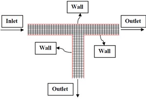
a)
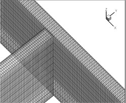
b)
Fig. 3The water flow in 3D geometry a) and flow velocity in x direction b)
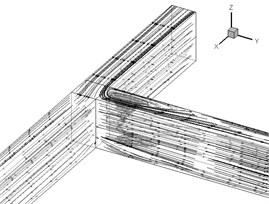
a)
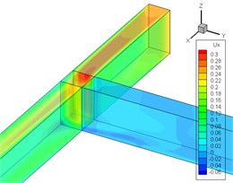
b)
6. Comparison of numerical and experimental models
In this section and the next three parts the effect of various turbulence models on flow velocity field, turbulence kinetic energy and the distribution of hydrostatic pressure at different sections of the main channel and intake for the input discharge of 0.011 cubic meters per second, the intake discharge rate () 0.31 and the Froude number of 0.13 are studied and their results are compared with the experimental results.
7. Comparing various turbulence models on flow velocity field
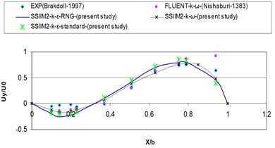
This section investigates the effect of various turbulence models on flow velocity profile at different sections of the main channel and intake. , and are obtained by dividing , and per the channel width (b). Fig. 3 shows the water flow in 3D geometry. According to Fig. 3, Fig. 4 shows velocity profile () near the surface for different cross sections of the main channel. is the maximum velocity of the cross section –4.65 the value of which equals 0.257 m/s.
Fig. 4Comparing computational velocity profile in the numerical and experimental modes
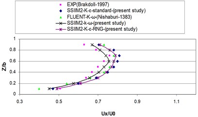
a)1
b)2
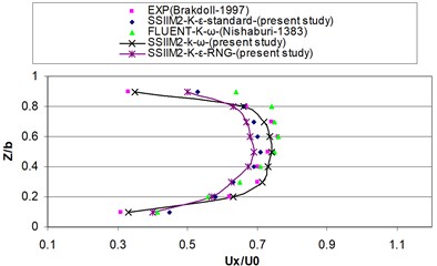
Fig. 5Comparing computational velocity profile in the numerical and experimental modes
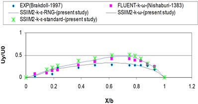
a)1
b)2.1
According to Fig. 5 the velocity retains its expanded state until a distance before the inlet and by approaching the inlet the velocity profiles are diverted into the branching channel due to the vacuum pressure applied by the intake and the maximum velocity is transformed into the inlet (point –0.5). According to the results of previous studies [9], the results of this research showed that by the entrance of the flow into the intake, the resultant velocity has decreased over the inlet and the maximum velocity recedes the inner wall of the main channel in the downstream input wall (point 0.5). The remaining flow within the channel after passing the intake inlet is developed in the section but due to the effects of the curvature of streamlines in the inlet, the maximum velocity is diverted toward the inside wall again. Fig. 5 also presents the dimensionless velocity profile () near the water surface for the cross sections of the intake channel. As you can see the - turbulence model has shown a better performance in estimating velocity than the other two - turbulence models and the positive and negative values of velocity show a relatively good agreement with the experimental results. The reason for this is the weakness - model in the secondary flow prediction due to the isotropic vortex viscosity.
The reason of the high values of predicted velocity values compared to the experimental results is the effects of secondary flow that transfer the maximum velocity to the lower levels of water. Tables 2 and 3 present the error percentage of comparing the flow velocity profile at different cross sections in the main channel and the intake in various turbulence models of --standard, --RNG and - in numerical and experimental modes.
Table 2Error percentage of comparing the flow velocity profile at different cross sections of the channel with experimental values in K-ε turbulence model
Cross-sections | ||||||||||||
–4.65 | –0.5 | 0 | 0.5 | 1 | 2 | 1 | 2.1 | 2.5 | 3 | 4 | 10 | |
Minimum error (%) | 5.5 | 1.6 | 2.4 | 2.1 | 2.7 | 2.8 | 18 | 5 | 2 | 2.7 | 8 | 4.7 |
The maximum error (%) | 15 | 15.1 | 30.1 | 21.3 | 24 | 10 | 39 | 42 | 44 | 40 | 41.5 | 35 |
Average error (%) | 8.4 | 7.1 | 18.1 | 14.7 | 15.9 | 6.5 | 25.4 | 24 | 21 | 32.4 | 43.3 | 18.9 |
Table 3Error percentage of comparing the flow velocity profile at different cross sections of the channel with experimental values in K-ε-RNG turbulence model
Cross-section | ||||||||||||
–4.65 | –0.5 | 0 | 0.5 | 1 | 2 | 1 | 2.1 | 2.5 | 3 | 4 | 10 | |
Minimum error (%) | 1.5 | 1.1 | 3.5 | 3.9 | 3.9 | 4.2 | 9 | 6.5 | 1.3 | 2.5 | 7.4 | 4.5 |
The maximum error (%) | 11.7 | 6 | 24.6 | 14.9 | 11.2 | 34 | 38 | 35 | 31 | 40 | 51 | 31 |
Average error (%) | 5 | 3.4 | 11 | 11.1 | 8.5 | 15.7 | 22 | 20 | 19 | 30 | 40 | 16.8 |
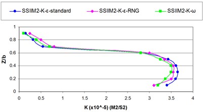
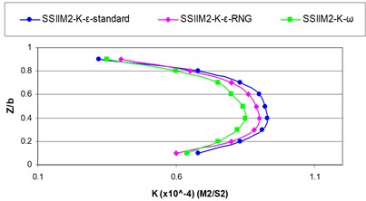
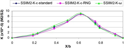
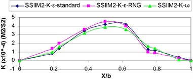
8. Comparing various turbulence models on turbulence kinetic energy
This section examines the effect of various turbulence models on, turbulence kinetic energy distribution at different sections of the main channel and intake. Figs. (6) and (7) show the turbulence kinetic energy () for various turbulence models in the main channel and intake in different turbulence models.
Fig. 6Comparing computational turbulence kinetic energy profile in the numerical and experimental modes
a)–4.65
b)1
Fig. 7Comparing computational turbulence kinetic energy profile in the numerical and experimental modes
a) 1
b) 3
As shown in the above figures by approaching the inlet due to the vacuum pressure applied by the intake the reduced velocity and turbulence value appear and the turbulence kinetic energy values are reduced and the turbulence kinetic energy diagrams loose their expanded state and divert into the intake inlet.
As the flow enters the intake inlet since the resultant velocity is reduced within the intake inlet, the turbulence kinetic energy is reduced and the maximum turbulence kinetic energy recedes the inner wall of the main channel in the downstream of the inlet wall.
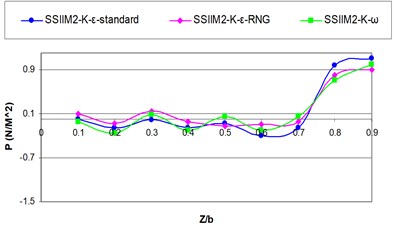
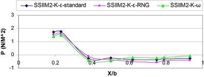
9. Comparing various turbulence models on hydrostatic pressure distribution
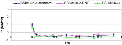
This section examines the effect of various turbulence models on, hydrostatic pressure distribution in different sections of the main channel. Figs. 8 and 9 present hydrostatic pressure distribution () for various cross sections of the main channel and the intake () in different turbulence models.
Fig. 8Comparing computational hydrostatic pressure distribution profile
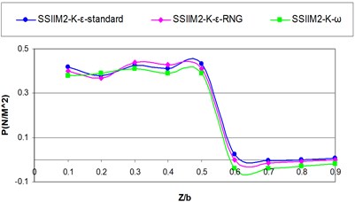
a)–0.5
a)1
Fig. 9Comparing computational hydrostatic pressure distribution profile
a) 1
b) 10
According to Fig. 9, before the intake inlet, the hydrostatic pressure distribution profile has a relatively constant trend but by approaching the inlet due to the applied vacuum pressure and the turbulent flow in the inlet the diagram experiences a sudden drop of pressure and the numerical value of the pressure becomes negative and as the flow gets away from the inlet the pressure distribution diagram experiences its former state.
10. Conclusions
- standard and the --RNG turbulence models are weak in predicting the flow velocity profile and the rotational region inside the intake but the - turbulence model shows a better performance due to the ability to predict the flows with low Reynolds number, absence of wall function and the prediction of the areas affected by the adverse pressure gradient.
Along the main channel the values of the turbulence kinetic energy is higher in --standard turbulence model than the --RNG turbulence model, also these values are lower in the - turbulence model than the other turbulence models along the main channel.
In a distance before the intake inlet the he hydrostatic pressure distribution profile has a relatively constant trend but by approaching the inlet due to the applied vacuum pressure and the turbulent flow in the inlet the diagram experiences a sudden drop of pressure and the numerical value of the pressure becomes negative.
References
-
Taylor E. H. Flow characteristics at rectangular open-channel junctions. Transactions of ASCE, Vol. 109, 1944, p. 893-902.
-
Law Reynolds Dividing flow in an open channel. ASCE, Vol. 192, Issue 2, 1966, p. 207-231.
-
Barkdoll B. D., Hagen B. L., Odgaard A. J. Laboratory Comparison of dividing open channel with duct flow in T-junction. Journal of Hydraulic Engineering ASCE, Vol. 124, Issue 1, 1998, p. 92-95.
-
Ramamurthy A. S., Junying Q. U., et al. Numerical and laboratory study of dividing open-channels flows. Journal of Hydraulic Engineering, Vol. 133, Issue 10, 2007, p. 1135-1144.
-
Neary V., Sotiropoulos F., OdgaardA. J. Three-dimensional numerical model of lateral-intake inflows. Journal of Hydraulic Engineering ASCE, Vol. 125, Issue 2, 1996, p. 126-140.
-
Issa R. I., Oliveira P. J. Numerical prediction of phase separation in tow-phase flow through T-Junctions. Computers and Fluids – Journal, Vol. 23, Issue 2, 1994, p. 347-372.
-
Pirzadeh B. Numerical investigation of velocity field in dividing open-channel flow. 12th WSEAS International Conference on Applied Mathematics, 2007, p. 195-198.
-
Olsen N. B. R. A three-dimensional numerical model for simulation of sediment movements in water intakes with moltiblock option. Department of Hydraulic and Environmental Engineering, the Norwegian University of Science and Technology, 2006.
-
Hsu Chung-Chieh, Tang Chii, Jau Lee, Wen-Jung, Shieh Mon-Yi Subcritical 900 equal-width open channel dividing flow. Journal of Hydraulic Engineering ASCE, Vol. 128, Issue 7, 2002, p. 716-720.
About this article

