Abstract
The paper firstly conducted a numerical simulation for flow fields and aerodynamic noises of the lateral window region in vehicles, and verified its correctness using the experimental test. Numerical simulation shows that: A pillar has a complicated shape and large corner, so that airflows will be separated here. An eddy structure is caused in the lateral window region and develops along the A pillar to generate serious pressure pulsations. A low pressure region is formed behind the A pillar. Obvious airflow separation regions are in the A pillar, rear view mirrors, wheels and wheel chambers. These airflow separation regions are typical positions causing aerodynamic noises. Additionally, large separated regions are located at the tail part of the vehicle, which is a main reason for causing the aerodynamic resistance. Intensity and velocity of eddies near the lateral window surface are relatively large, while its intensity near edges of the rear view mirror is weak. The shape of eddies extends along the flow direction to be an oval shape. The separated and broken eddies are sources for causing pressure pulsations. According to sound pressures of observation points, it can be also found that the separated eddy is a main reason for causing aerodynamic noises. Sound pressures are low at the right upper corner of lateral windows. In addition, noise distributions on the lateral window become gradually uniform with the increased frequency. In order to reduce flow noises, a bionic saw-tooth structure is applied to A pillars and rear view mirrors. After the bionic structure is introduced, some fluids are adhered to A pillars and rear view mirrors, so that the energy of fluids reaching the lateral window is reduced. In addition, fluids in rear regions of the rear view mirror presented a spiral shape, so that the possibility of fluid diffusion will be also reduced. In the original model, the maximum energy is 57.77, while that in this region with the bionic saw-tooth structures is 55.00. Obviously, the eddy energy is weakened. Compared with the original model, flow noises of all the observation points are reduced to different degrees, and the noise reduction effect is obvious. The results fully prove that this region with bionic saw-teeth in this paper has obvious advantages in noise reduction.
1. Introduction
When a vehicle is running at a high speed, aerodynamic noises will make the greatest contribution to the interior noise in vehicles [1-3]. Therefore, it will decide comfort of the vehicle [4-6]. Due to irregular surfaces and structures on the vehicle, high-speed airflows will cause a serious separation phenomenon while passing the outer surface of the vehicle, so that a complicated turbulent flow structure will be caused. Finally, strong pressure pulsations and aerodynamic noises will be generated in the front lateral window region, as shown in Fig. 1. The transmission loss in this region is very small, so that pressure pulsations and aerodynamic noises outside the vehicle will affect the comfort more easily. Therefore, it is very important to study aerodynamic noises in the lateral window region. The aerodynamic noise source near the front lateral window is caused by the A pillar-rear view mirror region.
Fig. 1Noise sources on the vehicle surface tested by the wind tunnel [7]
![Noise sources on the vehicle surface tested by the wind tunnel [7]](https://static-01.extrica.com/articles/18754/18754-img1.jpg)
At present, most of reported researches are mainly focused on aerodynamic noises of the rear view mirror or A pillar [8-13]. Alam [14] used a simplified model to conduct the wind tunnel test on several different A pillars in order to analyze impacts of geometric shapes on flow fields and aerodynamic noises of the vehicle. Levy [15] analyzed eddies caused by the airflow separation of the A pillar, and obtained relations between pulsation pressures and flow fields. Murad [11] used computational fluid dynamics software to simulate aerodynamic noises of the A pillar in a simplified vehicle model and studied impacts of flow velocities and yaw angles on aerodynamic noises of the A pillar. Hoarau [16] studied unsteady pressure fields of the A pillar combining LDV measurements with multi-point pressure measurements using off-set microphones. These reported researches on aerodynamic noises of the rear view mirror are more mature than those of the A pillar. Kato [17] adopted a simplified rear view mirror model, fixed it on a panel to complete wind tunnel tests, laying a reliable foundation for studying aerodynamic noises of bluff bodies. Khalighi [8] and Kim [18] studied flow fields on the tail part of the rear view mirror. Studied results show that eddies will appear alternately on the tail part of the rear view mirror; these eddies are pushed backwards along the airflow direction and weakened gradually; a long turbulent flow structure is formed in the rear region. Chen [19] conducted a numerical simulation of rear view mirrors with different edges. Studied results show that the edge will affect the velocity and streamline direction of airflows which flow through the rear view mirror cover to a great extent.
However, researches on aerodynamic noises for the complete A pillar-rear view mirror region are rarely reported. Based on eddy sound equations, Wang [20] analyzed relations between eddy vectors in flow fields near the A pillar and aerodynamic noses, and found main aerodynamic parameters which affected aerodynamic noises of the A pillar and rear view mirrors. However, the studied results are not verified by the experimental test. Yang [21] computed unsteady flow fields outside a passenger vehicle and aerodynamic noises in its lateral window region, and applied experimental PIV (particle image velocimetry) results to verify the correctness of the numerical simulation, but failed to conduct in-depth researches on lateral window regions. Regarding shortcomings in reported researches, this paper firstly conducted a numerical computation for flow fields and aerodynamic noises of the lateral window region, and verified the correctness of computational results.
2. Computational methods and models
2.1. Mathematic models
A DES (Detached Eddy Simulation) method provided by the commercial CFD software is used to solve non-steady flow characteristics outside the vehicle and flow fields in the lateral window region. The computational amount is lower than LES (Large Eddy Simulation) method. Non-steady flow characteristics which are more reliable than those computed by RANS (Reynolds-Averaged Navier-Stokes) can be obtained. Main idea of the DES method is to combine RANS with LES. The RANS method is applied to near-wall regions and the regions of which turbulence scale is smaller than the mesh size. The LES method is applied to regions outside the near wall region and the regions of which turbulence scale is larger than the mesh size. Its requirement for meshes is not higher than that of the LES method, so the computational amount can be reduced significantly. The DES method is to adopt a uniform eddy viscosity equation, where the mesh scale is used to distinguish RANS regions and LES regions, and then two models are used to solve the problem. In this paper, the DES method based on a - model is adopted, where equation and equation are as follows:
Eddy viscosity coefficient is determined by Eq. (3):
where: and are turbulence generation items, where their definitions and values of relevant coefficients in this model can be obtained in reference [22]. The expression of turbulence scale parameter in the equation dissipation item is as follows:
where: 0.09 and it is a model constant. In the DES method, the resolution scale in RANS and LES are defined by the following equation:
The coefficient 0.78. is the mesh scale. For non-uniform meshes, (, , ). In a boundary layer near the wall face, . The model is equivalent to a - turbulence model in RANS. When the distance is far away from the wall face, . The model is equivalent to a sub-grid stress model in LES. Compared with - model, the - model has the advantage that it is suitable to near-wall processing under a low Reynolds number. The - model considers shear stress transport. It does not contain any items similar to a complicated nonlinear viscosity attenuation item in the - model. Therefore, it is more suitable for computing flow fields of the vehicle with the detached characteristics [23]. In the computation, 0.615 and 4.306.
2.2. Geometric models
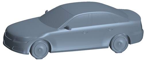
In the case of that the computational accuracy was not affected, the vehicle body was simplified; components including vehicle lamps and antenna were deleted; the vehicle bottom was simplified into a plane; wheels were simplified; wheel hubs and tread patterns were deleted, as shown in Fig. 2. When geometric simplification and cleaning of the complete vehicle model were conducted, the following situation was taken into account: due to impacts of shape characteristics of vehicle accessories and real vehicle bottom on flow fields, airflows near the vehicle body and the chassis were different from actual airflows, so the simulated accuracy was influenced. Therefore, when the simplification and cleaning of the vehicle accessories and the chassis were conducted, most shape characteristics of the vehicle accessories and chassis were reserved. Length is 4.68 m; width is 2.03 m; height is 1.44 m.
Fig. 2Geometric model of the processed vehicle
2.3. Mesh divisions
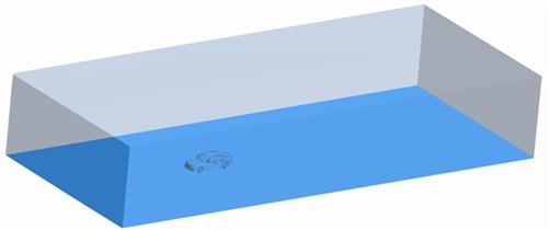
The computational domain is a cuboid enclosing the vehicle model, with length of 11 L, width of 5 W, height of 5 H, as shown in Fig. 3. The computational accuracy depends on the size of computational meshes. Meshes with the smaller size can touch the vehicle surface better, but will also increase a huge amount of meshes and long computational time. Due to limit in computer hardware, meshes may not be generated. Therefore, in sensitive regions on the vehicle surface, parameters have a large change gradient, and meshes should be fine, so that the accuracy of data transmission can be ensured.
Fig. 3Computational domain of flow fields of the vehicle
In general, computational results are deemed to be unrelated with meshes when the computational error of two sets of meshes is lower than 2 % [24-27]. For the model established in this paper, three sets of meshes are used for the trial computation. Results are shown in Table 1. Amounts of computational meshes are 5.6 million, 6.7 million and 7.3 million, respectively. It is found that the computational error is less than 1.59 % when the total amount of meshes is more than 7.3 million.
Table 1Comparison of computational results of three sets of meshes
Schemes | Maximum field mesh (mm) | Maximum surface mesh (mm) | Total amount of meshes / ×10,000 | Pressure value at observation points (Pa) | Relative errors |
1 | 30 | 12 | 560 | 595.2 | |
2 | 26 | 9 | 670 | 616.1 | 3.51 % |
3 | 22 | 6 | 730 | 625.9 | 1.59 % |
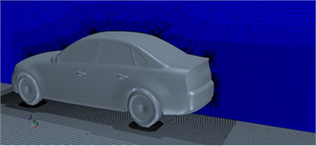
Therefore, the mesh amount in the computational model is 7.3 million, namely the maximum mesh size of the vehicle surface is 6 mm, which can satisfy requirements for mesh independence tests. Fig. 4 shows meshes in complete regions and local regions of the vehicle. Triangular meshes are established on the vehicle surface, where face meshes of the rear view mirror and base are the minimum with size of 2.5-5 mm. Size of face meshes of components including A pillar, B pillar and vehicle body waistline was 7.5 mm; size of face meshes on the lateral window is within 7.5-10 mm. Meshes on boundary layers are still adhered on the surfaces of rear view mirrors and vehicle body. The thickness of the first boundary layer is 0.1 mm. Growth rate and amount of the boundary layer are 1.15 and 12, respectively.
Fig. 4Meshes of the computational domain of the vehicle
a) Meshes on the longitudinal symmetric plane of the vehicle
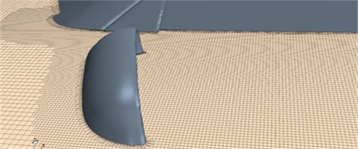
b) Local meshes around rear view mirrors
2.4. Boundary conditions
In the numerical simulation, Fluent was used to solve this problem. Due to the low flow velocity at the inlet, the incompressible flow was assumed here, and the density was set as a constant. In order to simulate aerodynamic noises of the vehicle more accurately, the computational method of Large Eddy Simulation (LES) was adopted in the turbulent flow computation. The Smagorinsky-Lilly model [28] was used as the sub-grid model of LES. The SIMPLEC algorithm was used to process the coupling between pressure and velocity. For boundary conditions, the inlet was set as the velocity inlet, uniform incoming flows were adopted, and 33.33 m/s was set as the inlet velocity and equivalent to 120 km/h; the outlet was set as the pressure outlet; the vehicle surface was a non-slippage face; in the computational domain, the upper surface and two sides were set as symmetric faces. The Reynolds average method was firstly used to obtain the initial steady solution. Then, the LES method was used for the computation. Time step length of aerodynamic noises could directly affect the computational frequency. In general, the sampling frequency is at least twice the optimal signal frequency. In view of the limited accuracy of CFD method in high frequency regions, 0.0001 s was set as the time step length; 10000 Hz was set as the sampling frequency; information within 5000 Hz can be obtained. In actual computation, a large time step length was used; when pressures at the observation point reached a steady state, the time step length was gradually reduced to 0.0001 s.
3. Results and discussions of the numerical simulation on flow fields
While flowing through the A pillar, airflows will get attached to the front lateral window and cause strong pressure pulsations, as shown in Fig. 5(a). Therefore, control measures for the A pillar will directly affect the downstream region of lateral windows. The lateral window is close to the A pillar, while the A pillar has a complicated shape and large corner, so that airflows will get separated obviously here. A part of the airflows flows through the connection between the A pillar and the front end of vehicles, and the other part of airflows passes through corner angles of A pillar and gets separated. Therefore, an eddy structure is formed in the lateral window region and develops backwards along the A pillar to cause large pressure pulsations. The flow velocity is high after the airflows flow through the A pillar and get separated. Therefore, a low pressure region is formed around the lateral window behind A pillar. Therefore, the eddy structure is caused by common effects between flow fields and wall faces. Due to the rear view mirror, pressure alternation becomes more complicated, and airflows at the front window become more chaotic. Similarly, the flow velocity of airflows in front of the rear view mirror is high, while the flow velocity of airflows behind the rear view mirror is low. Fluid velocities in wake flow regions of the rear view mirror were extracted for comparison, as shown in Fig. 6. It is shown in this figure that airflow velocities are low near the mirror face of rear view mirrors; obvious eddy structures will be generated in regions far from the mirror face. In addition, it can be found that eddies are in the wake flow region of the rear view mirror. Therefore, obvious eddies will be caused in the lateral window, and noises inside the vehicle will be also affected.
Fig. 5Velocity and pressure distributions in lateral window regions
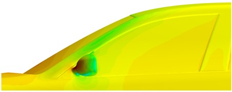
a) Distribution of pressure fields
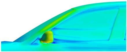
b) Distribution of velocity fields
Fig. 6Velocities in wake flow regions of rear view mirrors
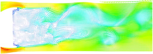
Fig. 7 shows positions and shapes of airflow separation regions described by contour surfaces with the total pressure 0 Pa. It is shown in this figure that obvious airflow separation regions are in the A pillar and rear view mirror regions. Large separation regions are also at wheels and wheel chambers. These airflow separation regions are typical positions causing aerodynamic noises. However, the reduction of aerodynamic noises can hardly be taken as design goals in shape design of wheels and vehicle bottom. In addition, large separated regions are at the tail part of the vehicle, which is a main reason causing aerodynamic resistance, but only affect aerodynamic noises in the vehicle slightly. In addition, it can be found that the airflows firstly get separated at the front lateral window region of the vehicle; then, a part of airflows gets attached in the rear lateral window region, while the other part of airflows gets attached in the front door handle.
Fig. 7Positions and shapes of airflow separation regions on vehicle surfaces
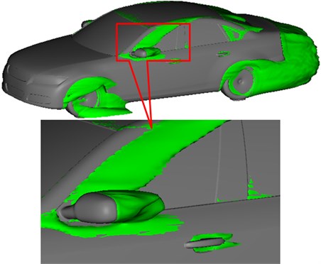
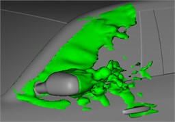
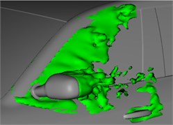
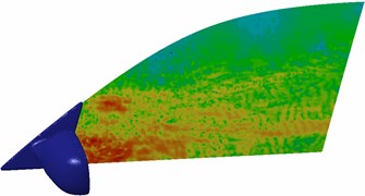
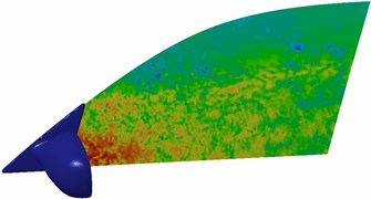
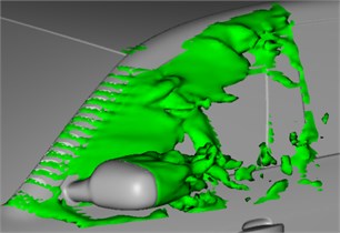
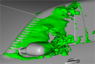
Fig. 8 shows two contour surfaces with internal 0.05 s and total pressure 0 Pa. The shape of the wake flow region of rear view mirrors changes obviously at the two moments, where changes of eddy regions in the A pillar are not obvious. The phenomena can be used to explain why aerodynamic noises generated in the wake flow region of rear view mirrors are more obvious in low frequency bands (below 750 Hz) compared with eddy regions of the A pillar. Eddy contour surfaces can be used to express spatial changes of velocities and reflect spatial unsteady eddy structures. Fig. 9 shows that: at the same 2 moments, eddies of the lateral window region are a contour surface shape of 1300 s-1, where different colors represent different sizes of airflow velocities. After airflows flow through the A pillar, one part of the separation fluid flows along the surface and edge of rear view mirrors; the other part flows through narrow space between the rear view mirror and the lateral window, gets accelerated and collided the lateral window; two parts of airflows form eddies behind the rear view mirror. They are formed through accelerated rotating motion of low-velocity airflows behind the rear view mirror under driving of high-velocity airflows which flow through the top part and lateral part of the rear view mirror. It can be found: eddy intensity and velocity near the lateral window surface are relatively large; eddy intensity near edges of the rear view mirror is relatively weak; the shape extends along the airflow direction to be an oval shape. One part of airflows passes through outer edges of the rear view mirror; the other part of airflows passes through narrow space between the lateral window surface and the rear view mirror. The two parts of airflows are similar to valves with different sizes. Under the same pressure and velocity of incoming flow, the smaller valve opening degree will cause higher flowing velocity of water flows. Therefore, the flowing velocity of airflows between the rear view mirror and the lateral window far is more than that of airflows flowing through outer edges of the rear view mirror. High-velocity airflows passing through narrow space between the rear view mirror and the lateral window will drive low-velocity airflows behind the rear view mirror to make strong rotation motion, and strong eddies are generated on the inner side of rear view mirrors. Eddies keep on developing to the downstream and get broken and dispersed. The separated and broken eddies are sources causing pressure pulsations. Airflows accelerated by the narrow space between the rear view mirror and the lateral window will obviously affect pressure distributions on the lateral window, so large pressure pulsations will be generated. For low-velocity jet flows, development and breaking of eddies are the main reasons causing aerodynamic noises.
Fig. 8Airflow separation status at different moments
a) 0.20 s
b) 0.25 s
Fig. 9Eddy contour surfaces of lateral window regions at different moments
a) 0.20 s
b) 0.25 s
4. Results and discussions of the numerical simulation on flow noises
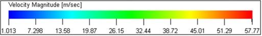
Airflow separation in lateral window regions will generate serious aerodynamic noises. The computation of aerodynamic noises is generally completed by finite element or boundary element methods. Regarding finite element method, the acoustic space generally needs to be dispersed into meshes. For boundary element method, the space only needs to be dispersed into shell meshes. The boundary element method can reduce dimensions of acoustic problems, so the computational amount can be decreased greatly. Meanwhile, the boundary element method is a semi-analytical numerical method which combines analysis and dispersion, and has high solution accuracy. In the flow field computation, structural meshes are divided finely and the model is large. If structural meshes are directly used as the boundary element model, the computational efficiency will be low, so that computational results and accuracy will not be increased obviously. In order to obtain ideal computation results, surface meshes are extracted based on the structural model. Actual geometric characteristics of the structure should be simulated accurately. Meanwhile, the mesh size should satisfy that each element length at least includes 6 sound wave wavelengths [29-33]. In this paper, 11 mm is selected as the mesh size; the boundary element model has 23089 elements; the maximum frequency is 5000 Hz. In order to observe aerodynamic noises in the lateral window region, 11 observation points are arranged, as shown in Fig. 10(a). The boundary element model is shown in Fig. 10(b).
Fig. 10Boundary element model and observation points
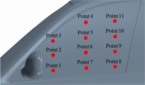
a)
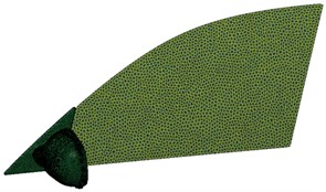
b)
Fig. 11 shows comparisons of sound pressure levels at each observation point. It is found that the observation point 3 had the maximum sound pressure level because this point is located at the wake flow region of the rear view mirror, with the largest eddy intensity. Sound pressure levels of other observation points are not very different because these points are located at the wake flow region of the rear view mirror, with small eddy intensity. When the analyzed frequency is less than 3000 Hz, sound pressure levels of each observation point are gradually decreased with the analyzed frequency. When the analyzed frequency is more than 3000 Hz, sound pressure levels of each observation point tend to reach a steady value. In addition, it is shown in Fig. 11(c) that sound pressure levels of observation points 10 and 11 are less than those of observation points 8 and 9. It is shown in Fig. 9 that observation points 8 and 9 are located at eddy regions of the lateral window; separated eddies are not at observation points 10 and 11. The phenomena can indicate that the separated eddy is a main reason causing aerodynamic noises.
Fig. 11Sound pressure levels of different observation points
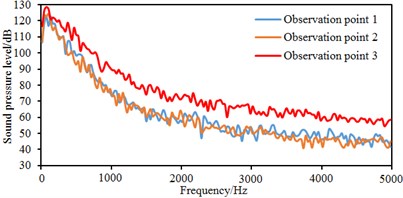
a) Observation points 1, 2, 3
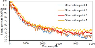
b) Observation points 4, 5, 6, 7
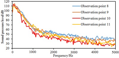
c) Observation points 8, 9, 10, 11
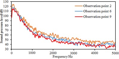
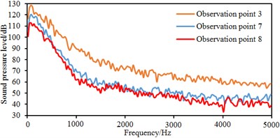
In order to observe changes of sound pressure levels on the same horizontal plane, sound pressure levels at observation points 2, 3, 6, 7, 8 and 9 are extracted for comparison, as shown in Fig. 12.
Fig. 12Sound pressure levels at the same horizontal panel
a) Observation points 2, 6, 9
b) Observation points 3, 7, 8
It is shown in Fig. 12(a) that sound pressure levels at observation points 2, 6 and 9 are basically consistent because the three observation points are located in longitudinal eddies on the lateral window surface. Sound pressure levels at observation point 2 are slightly higher than those at other two observation points because airflow separation is relatively serious and many broken eddies are at the observation point 2. It is shown in Fig. 12(b) that on the same horizontal plane, sound pressure levels at observation point 3 obviously are more than those at other two observation points because observation point 3 is located at the eddy center of the wake flow region of the rear view mirror and has a large eddy intensity. Similarly, sound pressure levels at observation point 7 are slightly higher than those at the observation point 8 because only a few of separation and broken eddies are at observation point 8.
Sound pressure contours at different frequencies were extracted, as shown in Fig. 13. Sound wave wavelengths are large at low frequencies, so that large eddy noises will be caused when sound waves hit the separated eddies. Sound wave wavelengths are short at high frequencies and sound waves can bypass the separated eddies, so only small eddy noises will be generated. Therefore, size of convex parts in the lateral window region is greatly more than the noise wavelength at high frequencies and noise sources are distributed more uniformly; on the contrary, the noise source distribution will become uneven. As a result, noise distributions on the lateral window surface become gradually uniform with the increased frequency. In addition, it can be found that sound pressures in the wake flow region near the rear view mirror are very large. The reason is that airflow separation phenomena are serious in the wake flow region near rear view mirrors, and sound pressures are obviously low at the right upper part of lateral windows. It is shown in Fig. 9 that separated and broken eddies do not appear at this position, and no eddy noises are caused.
Fig. 13Contours of sound pressures at different frequencies
a) 500 Hz
b) 2000 Hz
c) 3500 Hz
d) 5000 Hz
5. Experimental verification of flow noises
In the experimental test, the tested vehicle was located in front of the wind tunnel center. The surface microphones were used to collect sound pressure signals at 11 observation points which were arranged on the front lateral window. The surface microphones are precious and can be damaged easily [34-36], so they should be sleeved by nylon casings for protection, should be fixed by adhesive tapes, and should be prevented from shaking during the experimental test. Sensors should be kept flush with the lateral window glass, so that the accuracy of tested noises can be ensured. The experimental status was as follows: yaw angle of the vehicle was 0°; experimental wind velocity was 120 km/h; the motion belt was kept stationary; suction of boundary layers did not exist; lateral windows and doors were fully sealed by adhesive tapes. In this way, the experimental structure would be the same as the simulated structure. In addition, in order to observe airflows in the wake flow region of rear view mirrors, the laser particle image velocimetry technology (PIV) was used in the wind tunnel to test velocity fields in the wake flow region of rear view mirrors, as shown in Fig. 14, so the correctness of the numerical simulation method can be verified. A particle generator was placed at a stable section of the wind tunnel, so its interference to the original flow field could be reduced. The particle generator was started intermittently. Tracing particles passed through a wind tunnel honeycomb device and a damping net for rectification. Then, after one wind tunnel backflow cycle, the particles could be mixed uniformly with the air flow field, so flow states of the experimental wind tunnel section can be expressed fully. Background noises should be tested before the real test was conducted, so whether the background noise would form interference could be confirmed. After sensors were corrected, the wind source was opened, and the wind velocity was accelerated gradually. When the wind velocity reached 120 km/h and the airflow velocity in the experimental section reached a stable value, noise signals and velocity fields were collected and processed by computational software [37-40].
Fig. 14Laser particle image velocimetry technology
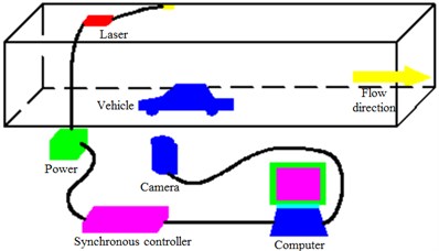
Fig. 15 shows the comparison between experimental test and numerical simulation of sound pressures at some observation points. It is shown in these figures that experimental and numerical simulation results have the consistent trends. When the analyzed frequency is less than 3000 Hz, the sound pressure is gradually decreased with the analyzed frequency. When the analyzed frequency is more than 3000 Hz, the sound pressure gradually tends to reach stable values. In addition, the maximum relative error between experimental test and numerical simulation is not more than 5 %. The results fully verify the correctness of the numerical model in this paper.
Fig. 15Comparisons of sound pressure levels between simulation and experiment
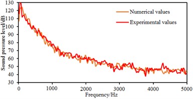
a) Observation point 2
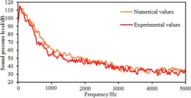
b) Observation point 5
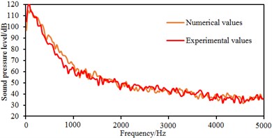
c) Observation point 9
In addition, velocity fields in the tail region of rear view mirrors obtained in experimental test were extracted and compared with numerical simulation results, as shown in Fig. 16. It is shown in Fig. 16 that velocity fields between experiment and simulation are also similar. Regions near the mirror face are low-velocity regions without any eddy. Obvious eddies are caused in regions far away from the mirror face. Experimental test and numerical simulation have the similar flow directions, where high-velocity regions are on the upper and lower sides of the flow domain, and the low-velocity regions are in the middle. The range of low-velocity regions is gradually narrowed and gets deviated towards the upper side. In addition, the maximum flow velocity of the numerical simulation is 58.40 m/s, and that of experimental test is 58.31 m/s. The difference is very small. The comparison can verify the correctness of the numerical model in this paper.
Fig. 16Comparisons of velocity fields between numerical simulation and experimental test
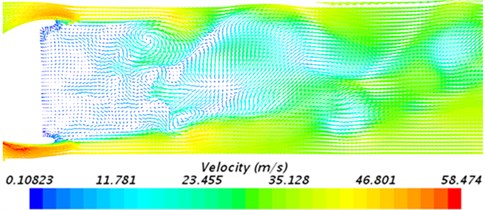
a) Numerical simulation
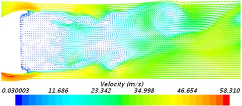
b) Experimental test
6. Control and optimization of flow noises
Flow fields and noise mechanisms of the lateral window region are introduced above. However, reported researches are rarely focused on noise reduction measures of the lateral window region. Most work is focused on studying the topological structure of eddies in this region. As one of the passive control methods for flow fields, a bionic structure can be applied to the lateral window region of an actual vehicle for the numerical simulation, so that its impacts on flow fields can be explored. Most researches on bionic noise reduction take the tyto alba as the object because it is a kind of bird with silent flying ability. Researchers point out that the tyto alba has the silent flying ability because other types of birds do not have the following three features: floppy fluff on wing surface and legs, fringe structures on the rear feather edge and saw-tooth structures on the front edge of primaries. Fig. 17 shows the micro-structure of wing feather of the tyto alba, where the feather front edge has a saw-tooth structure. Studied results show that the front-edge saw-tooth structure has similar functions to an eddy generator. In addition, it co-works with wing tip feather and front edge slat in order to reduce boundary layer separation on the surface, which plays a key role in reducing noises during flight. Therefore, the bionic saw-tooth structure is applied to the lateral window region, as shown in Fig. 18.
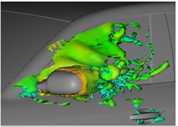
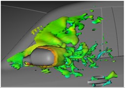
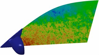
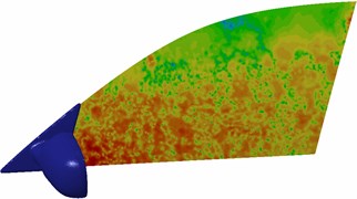
The bionic saw-tooth structure is applied to A pillars and rear view mirrors for computing of flow fields, as shown in Fig. 19 and Fig. 20. Fig. 19 shows two contour surfaces with interval 0.05 s and total pressure 0 Pa. Fig. 20 shows that: at the same 2 moments, vortexes of the lateral window region are a contour surface shape of 1300 s-1, where different colors represent different sizes of airflow velocities. It is shown in Fig. 19 and Fig. 20 that after setting some bionic saw-tooth structures on A pillars and rear view mirrors, some fluids are adhered to this region, so that the energy of fluids reaching the lateral window is reduced.
Fig. 17Micro-structure of feather in the tyto alba [41, 42]
![Micro-structure of feather in the tyto alba [41, 42]](https://static-01.extrica.com/articles/18754/18754-img32.jpg)
a)
![Micro-structure of feather in the tyto alba [41, 42]](https://static-01.extrica.com/articles/18754/18754-img33.jpg)
b)
![Micro-structure of feather in the tyto alba [41, 42]](https://static-01.extrica.com/articles/18754/18754-img34.jpg)
c)
Fig. 18Local model of the bionic structure in vehicles
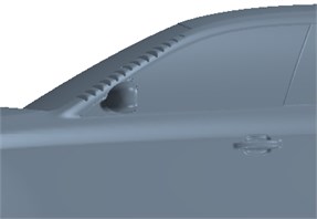
a)
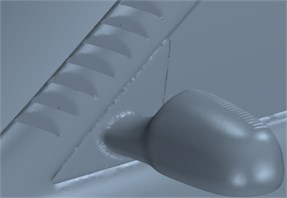
b)
In addition, it is also shown in Fig. 20 that fluids in rear regions of the rear view mirror presented a spiral shape, so that the possibility of fluid diffusion will be reduced. In Fig. 9, the maximum energy in this region is 57.77, while that in this region with the bionic saw-tooth structures is 55.00. Obviously, the eddy energy is weakened, which will further reduce flow noises in the region. In order to verify the conclusion, flow noises in the region were computed again. Limited by this paper length, noises of some observation points were extracted for comparison with the original structure. Results are shown in Fig. 21. It is shown in these figures that flow noises of all the observation points are reduced to different degrees. The noise reduction effect is obvious especially at observation point 11. The results fully prove that this region with bionic saw-teeth in this paper has obvious advantages in noise reduction.
Fig. 19Airflow separation states at different moments
a) 0.20 s
b) 0.25 s
Fig. 20Vortex contour surfaces of lateral window regions at different moments
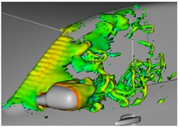
a) 0.20 s
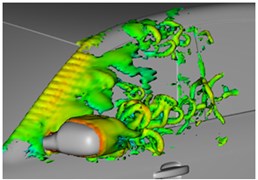
b) 0.25 s
Fig. 21Comparison of flow noises at observation points before and after optimization
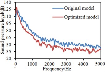
a) Observation point 1
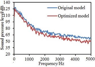
b) Observation point 3
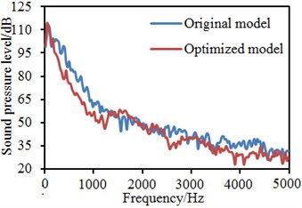
c) Observation point 5
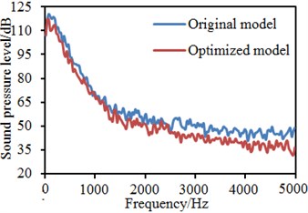
d) Observation point 7
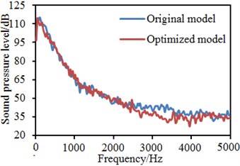
e) Observation point 9

f) Observation point 11
7. Conclusions
The paper firstly conducted a numerical computation for flow fields and aerodynamic noises of the lateral window region in vehicles, and verified its correctness using the experimental test. The following conclusions can be obtained:
1) The A pillar has a complicated shape and large corner, so that airflows will be separated here. A eddy structure is formed in the lateral window region and develops along the A pillar to cause large pressure pulsations. A low pressure region is caused behind the A pillar.
2) Eddy intensity and velocity near the lateral window surface are relatively large, while eddy intensity near edges of the rear view mirror is relatively weak. The shape of eddies extends along the airflow direction to be an oval shape. The separated and broken eddies are sources causing pressure pulsations and aerodynamic noises. Sound pressures are low at the right upper corner of lateral windows. In addition, noise distributions on the lateral window become gradually uniform with the increased frequency.
3) Experimental test and numerical simulation have a consistent change trend, and the maximum error is less than 5 %. Velocity fields are also similar between the experimental test and numerical simulation. Regions near the mirror face are low-velocity regions. Obvious eddies are generated at places far from the mirror face region. Flow directions are also similar, which further verifies the correctness of the computational model in this paper.
4) A bionic saw-tooth structure is applied to A pillars and rear view mirrors for reducing flow fields and noises. After the bionic saw-tooth structure is introduced into A pillars and rear view mirrors, some fluids are adhered to this region, so that the energy of fluids reaching the lateral window is reduced. In addition, fluids in rear regions of the rear view mirror presented a spiral shape, so that the possibility of fluid diffusion will be reduced. In the original model, the maximum energy in this region is 57.77, while that in this region with the bionic saw-tooth structures is 55.00. Obviously, the eddy energy is weakened. Finally, flow noises in the region were computed again. Compared with the original model, flow noises of all the observation points are reduced to different degrees, and the noise reduction effect is obvious. The results fully prove that this region with bionic saw-teeth in this paper has obvious advantages in noise reduction.
References
-
Papoutsis-Kiachagias E. M., Magoulas N., Mueller J., et al. Noise reduction in automobile aerodynamics using a surrogate objective function and the continuous adjoint method with wall functions. Computers and Fluids, Vol. 122, 2015, p. 223-232.
-
Li J., Deng G., Luo C., et al. A hybrid path planning method in unmanned air/ground vehicle (UAV/UGV) Cooperative systems. IEEE Transactions on Vehicular Technology, Vol. 65, Issue 12, 2016, p. 9585-9596.
-
[3]Huijssen J, Fiala P, Hallez R, et al. Numerical evaluation of source–receiver transfer functions with the fast multipole boundary element method for predicting pass-by noise levels of automotive vehicles. Journal of Sound and Vibration, Vol. 331, Issue 9, 2012, p. 2080-2096.
-
Duell E. G., Walter J., Yen J., et al. Progress in aero-acoustic and climatic wind tunnels for automotive wind noise and acoustic testing. SAE International Journal of Passenger Automobiles – Mechanical Systems, Vol. 6, 2013, p. 448-461.
-
Cui K., Yang W., Gou H. Experimental research and finite element analysis on the dynamic characteristics of concrete steel bridges with multi-cracks. Journal of Vibroengineering, Vol. 19, Issue 6, 2017, p. 4198-4209.
-
Huijssen J., Hallez R., Pluymers B., et al. A synthesis procedure for pass-by noise of automotive vehicles employing numerically evaluated source-receiver transfer functions. Journal of Sound and Vibration, Vol. 332, Issue 15, 2013, p. 3790-3802.
-
Cogotti A. Evolution of performance of an automotive wind tunnel. Journal of Wind Engineering and Industrial Aerodynamics, Vol. 96, Issue 6, 2008, p. 667-700.
-
Khalighi B., Chen K. H., Johnson J. P., et al. Computational and experimental investigation of the unsteady flow structures around automotive outside rear-view mirrors. International Journal of Automotive Technology, Vol. 14, Issue 1, 2013, p. 143.
-
Khalighi B., Snegirev A., Shinder J., et al. Simulations of flow and noise generated by automobile outside rear-view mirrors. International Journal of Aeroacoustics, Vol. 11, Issue 1, 2012, p. 137-156.
-
Wei W., Fan X., Song H., et al. Imperfect information dynamic stackelberg game based resource allocation using hidden Markov for cloud computing. IEEE Transactions on Services Computing, Vol. 99, 2016, p. 1-13.
-
Murad N., Naser J., Alam F., et al. Computational fluid dynamics study of vehicle A-pillar aero-acoustics. Applied Acoustics, Vol. 74, Issue 6, 2013, p. 882-896.
-
Murad N. M., Naser J., Alam F., et al. A computational fluid dynamics study of crosswind effects on vehicle A-pillar aero-acoustics. International Journal of Vehicle Noise and Vibration, Vol. 9, Issues 3-4, 2013, p. 147-170.
-
Levy B., Brancher P. Experimental investigation of the wall dynamics of the A-pillar vortex flow. Journal of Fluids and Structures, Vol. 55, 2015, p. 540-545.
-
Alam F., Watkins S., Zimmer G. Effects of vehicle A-pillar shape on local mean and time-varying flow properties. SAE Paper 2001-01-1086, 2001.
-
Levy B., Brancher P. Topology and dynamics of the A-pillar vortex. Physics of Fluids, Vol. 25, Issue 3, 2013, p. 037102.
-
Hoarau C., Borée J., Laumonier J., et al. Unsteady wall pressure field of a model A-pillar conical vortex. International Journal of Heat and Fluid Flow, Vol. 29, Issue 3, 2008, p. 812-819.
-
Kato Y. Numerical simulations of aeroacoustic fields around automobile rear-view mirrors. SAE International Journal of Passenger Automobiles-Mechanical Systems, Vol. 5, 2012, p. 567-579.
-
Jeong-Hyun K., Yong O. H. Experimental investigation of wake structure around an external rear view mirror of a passenger automobile. Journal of Wind Engineering and Industrial Aerodynamics, Vol. 99, Issue 12, 2011, p. 1197-1206.
-
Chen X., Wang H. Y., Gao C. F., Zhang W., Xie C. Effect of rearview mirror edge structure on flow field and aerodynamic noise. Journal of Aerospace Power, Vol. 29, Issue 5, 2014, p. 1099-1104.
-
Wang Y. G., Huang X. S., Wei W., Yang Z. G. Aerodynamic noise optimization of vehicle’s A-pillar based on vortex sound theory. Noise and Vibration Control, Vol. 37, Issue 2, 2017, p. 107-112.
-
Yang B., Hu X. J., Wang F. L. Numerical simulation and verification of aerodynamic noise from side window region of minivan. Journal of Jilin University (Engineering and Technology Edition), Vol. 40, Issue 4, 2010, p. 915-919.
-
Menter F. Zonal k-ω two equation turbulence models for aerodynamic flow. 24th Fluid Dynamics Conference, Orlando, AIAA-93-2906, USA, 1993.
-
Wu J., Gu Z. Q., Zhong Z. H. The application of SST turbulence model in the aerodynamic simulation of the automobile. Automotive Engineering, Vol. 25, Issue 4, 2003, p. 326-329.
-
Onkarappa N., Sappa A. D. Synthetic sequences and ground-truth flow field generation for algorithm validation. Multimedia Tools and Applications, Vol. 74, Issue 9, 2015, p. 3121-3135.
-
Niu J., Liang X., Zhou D. Experimental study on the effect of Reynolds number on aerodynamic performance of high-speed train with and without yaw angle. Journal of Wind Engineering and Industrial Aerodynamics, Vol. 157, 2016, p. 36-46.
-
Yang A., Han Y., Pan Y., et al. Optimum surface roughness prediction for titanium alloy by adopting response surface methodology. Results in Physics, Vol. 7, 2017, p. 1046-1050.
-
García J., Muñoz-Paniagua J., Jiménez A., et al. Numerical study of the influence of synthetic turbulent inflow conditions on the aerodynamics of a train. Journal of Fluids and Structures, Vol. 56, 2015, p. 134-151.
-
Shi Z., Chen J., Chen Q. On the turbulence models and turbulent Schmidt number in simulating stratified flows. Journal of Building Performance Simulation, Vol. 9, Issue 2, 2016, p. 134-148.
-
Opperwall T., Vacca A. A combined FEM/BEM model and experimental investigation into the effects of fluid-borne noise sources on the air-borne noise generated by hydraulic pumps and motors. Proceedings of the Institution of Mechanical Engineers, Part C: Journal of Mechanical Engineering Science, Vol. 228, Issue 3, 2014, p. 457-471.
-
Xiao P., Wu J. S., Cowan C. F. N. MIMO detection schemes with interference and noise estimation enhancement. IEEE Transactions on Communications, Vol. 59, Issue 1, 2011, p. 26-32.
-
Mallardo V., Aliabadi M. H., Brancati A., et al. An accelerated BEM for simulation of noise control in the aircraft cabin. Aerospace Science and Technology, Vol. 23, Issue 1, 2012, p. 418-428.
-
Cui K., Zhao T. T. Unsaturated dynamic constitutive model under cyclic loading. Cluster Computing, 2017, p. 1-11, https://doi.org/10.1007/s10586-017-0881-9.
-
Larbi W., Deü J. F., Ohayon R., et al. Coupled FEM/BEM for control of noise radiation and sound transmission using piezoelectric shunt damping. Applied Acoustics, Vol. 86, 2014, p. 146-153.
-
Li J. Q., He S. Q., Ming Z. An intelligent wireless sensor networks system with multiple serves communication. International Journal of Distributed Sensor Networks, Vol. 7, 2015, p. 1-9.
-
Cui K., Qin X. Virtual reality research of the dynamic characteristics of soft soil under metro vibration loads based on BP neural networks. Neural Computing and Applications, 2017, p. 1-10, https://doi.org/10.1007/s00521-017-2853-7.
-
Wei W., Song H., Li W., et al. Gradient-driven parking navigation using a continuous information potential field based on wireless sensor network. Information Sciences, Vol. 408, 2017, p. 100-114.
-
Du J., Xiao P., Wu J., et al. Design of isotropic orthogonal transform algorithm-based multicarrier systems with blind channel estimation. IET Communications, Vol. 6, Issue 16, 2012, p. 2695-2704.
-
Wu J. S., Blostein S. D. High-rate diversity across time and frequency using linear dispersion. IEEE Transactions on Communications, Vol. 56, Issue 9, 2008, p. 1469-1477.
-
Ding G., Tan Z. Indoor fingerprinting localization and tracking system using particle swarm optimization and Kalman filter. IEICE Transactions on Communications, Vol. 98, Issue 3, 2015, p. 502-514.
-
Li J., Yu F. R., Deng G., et al. Industrial Internet: A survey on the enabling technologies, applications, and challenges. IEEE Communications Surveys and Tutorials, Vol. 19, Issue 3, 2017, p. 1504-1526.
-
Bachmann T., Klän S., Baumgartner W., et al. Morphometric characterisation of wing feathers of the barn owl Tyto alba pratincola and the pigeon Columba livia. Frontiers in Zoology, Vol. 4, 2007, p. 1-23.
-
Bachmann T., Wagner H. The three-dimensional shape of serrations at barn owl wings: towards a typical natural serration as a role model for biomimetic applications. Journal of Anatomy, Vol. 219, Issue 2, 2011, p. 192-202.
About this article

