Large-eddy simulations of the inlet grid-generated turbulence

Zhiwei, Zhang; Bo, Wu; Liangliang, Zhang; Yuanqing, Wang; Longxian, Huang

doi:10.21595/vp.2020.21370

Vibroengineering Procedia

Browse Procedia

Published: 02 April 2020

Check for updates

Large-eddy simulations of the inlet grid-generated turbulence

Zhang Zhiwei¹

Wu Bo²

Zhang Liangliang³

Wang Yuanqing⁴

Huang Longxian⁵

^{1, 2}School of Civil Engineering, Chongqing University, Chongqing, 400045, China

³City College of Science and Technology, Chongqing University, Chongqing, 400045, China

⁴The 5th Engineering Co., Ltd of China Railway 11th Bureau Group, Chongqing, 400037, China

⁵Chongqing Expressway Co., Ltd, Chongqing, 401121, China

Corresponding Author:

Wu Bo

Cite the article Download PDF

Downloads 1200

CrossRef Citations 1

Abstract

In this paper, a new technique of turbulence generation in large eddy simulation (LES) is studied and verified. In order to generate turbulence similar to the wind tunnel test, the proposed grid inlet technique places the grid on the Inlet boundary to achieve the following effects: changing the grid size controls the turbulence integral length scale and changing the distance from inlet controls the turbulence intensity. The purpose of this paper is to explore the domain requirements of grid-inlet technology by studying the turbulence characteristics of three different grid inlets. In particular, this paper further studies the effects of domain sizes on the lateral correlation of fluctuating wind by arranging the transverse positions of monitoring points irregularly and in equal proportion. Meanwhile, the isotropic hypothesis of gird-generated turbulence is verified by power spectrum. The results show that the turbulence intensity is unaffected by the domain sizes, the larger calculation domain corresponds to the gentler changing trend of the lateral correlation of the fluctuating wind and the flow fields under the three different domain sizes basically satisfy the isotropic hypothesis. The above results are helpful for the further application of the grid inlet technique.

1. Introduction

Grids are typically used to experimentally generate flows with different turbulence characteristics. At present, large eddy simulation is the best method to generate turbulence. In Large Eddy Simulation, the description of turbulence characteristics is a well-known problem due to the instabilities of turbulence vortices and their temporal and spatial correlations [1]. Pre-computation methods and synthetic inlet methods are the two typical methods to generate turbulence in In Large Eddy Simulation.

In the pre-computation method, a streamwise cyclic boundary is used to make the flow circulate on the boundary. Time data is kept in a library for application to the inlet in further simulations. Because of the time and storage required, this method is not efficient. In order to avoid the possible introduction of fictitious periodicity, shorter phase jitter pre-computation is recommended [2]. However, to let the flow evolve into ‘real’ turbulence, a considerable simulation inlet length was found to be required. DeVilliers [3] describes a more efficient time and data storage method in which internal mapping planes are used to recover flow upstream of the main computational domain. In this method, there is no need to store pre-calculated data. In most pre-computation methods, it is almost impossible to generate turbulence with the specific length scale and turbulence intensity, due to the limitations of boundary layer of the domain geometry.

Carati [4] and Wang [5] studied free decaying homogeneous isotropic turbulence by synthesizing turbulence. Through modifying a random field to adapt a specified spectrum, the initial condition is generated at a single point in time. This is relatively uncomplicated, but when synthesizing inlet turbulence which is also correlated in time, difficulty begins to arise. The simplest form of a synthetic inlet is to superpose a random fluctuation on the average flow. And the fluctuations do not have structure and dissipate quickly because they are not correlated [1]. Smirnov et al. [6] operated a random field to meet continuity requirements and generate a more precise description of turbulence. However, this method still does not offer satisfactory control when generating “real” turbulence. Davidson [7] and Fathali et al. [8] put forward a more advanced synthetic inlet method in which correlation filters are applied to random fields to generate turbulence with specific turbulence characteristics. However, it has been demonstrated that a reasonable inlet length is still necessary to generate turbulence with specific turbulence characteristics [1]. It is therefore difficult to generate high-intensity turbulence through synthetic inlet methods due to turbulence dissipation.

After analyzing and comparing the above two turbulence generating methods, Tabor and Baba-Ahmadi [1] put forward that the most efficient turbulence generating method in LES was the internal mapping method. Based on this conclusion, a new technique of turbulence generation is proposed in which the solid patches are placed on the Inlet boundary.

By using the proposed new method, this paper develops turbulence using the projected pattern of a grid on the inlet boundary to generate grid turbulence as used in wind tunnel tests. The grid-generated turbulence has the following characteristics: changing the grid size controls the turbulence integral length scale and changing the distance from inlet controls the turbulence intensity [9]. The purpose of this paper is to explore the domain requirements of grid-inlet technology by studying the turbulence characteristics of three different grid inlets.

2. Numerical model and basic methods

2.1. Governing equations and numerical algorithm

In this paper, numerical simulations are carried out by solving the three-dimensional unsteady incompressible governing equations of the ﬂuids. The ﬁltered continuity and Navier-Stokes equations for 3D LES with the SGS model are shown in Eq. (1). In the equations, the grid-scale turbulence is solved while the sub-grid-scale turbulence is modeled:

1

\frac{\partial {\bar{u}}_{i}}{\partial x_{i}} = 0, \frac{\partial ({\bar{u}}_{i})}{\partial t} + \frac{\partial ({\bar{u}}_{i} {\bar{u}}_{j})}{\partial x_{j}} = - \frac{1}{ρ} \frac{\partial \bar{p}}{\partial x_{i}} + μ \frac{\partial^{2} {\bar{u}}_{i}}{\partial x_{i} \partial x_{j}} - \frac{\partial τ_{i j}}{\partial x_{j}},

where $u_{i}$ and $x_{i}$ ( $i =$ 1, 2, 3) are the three velocity and displacement components; $t$ , $ρ$ , $p$ , and $μ$ are time, density, pressure, and kinematic viscosity. The over-bar represents filtered field variable. $τ_{i j}$ , $τ_{i j} = \bar{u_{i} u_{j}} - {\bar{u}}_{i} {\bar{u}}_{j}$ , is the sub-grid scale stress (SGS) , which is the product of the spatial filtration of the fluid equation and the energy exchange link between the solvable scale and the sub-grid scale, as expressed in Eq. (5):

2

τ_{i j} - \frac{1}{3} δ_{i j} τ_{k k} = - 2 ν_{S G S} {\bar{S}}_{i j} = ν_{S G S} (\frac{\partial {\bar{u}}_{i}}{\partial x_{j}} + \frac{\partial {\bar{u}}_{j}}{\partial x_{i}}),

where ${\bar{S}}_{i j}$ is the strain rate tensor and $ν_{S G S}$ is the SGS eddy viscosity $ν_{S G S} = {(C_{S} \bar{Δ})}^{2} |\bar{S}|$ , where $C_{S}$ is the Smagorinsky coefficient.

In the present study, simulations were run by using the FLUENT CFD software to solve the discrete model. A time step of 0.001 was set. The number of time steps was set to 15000; in other words, the total length is 15 s. In the process of solving the LES control equation, the Second Order discrete scheme was used for the pressure term and the Bounded Central Differentiation scheme was used for the momentum term. The numerical method is the Simple algorithm, the transient term is solved by the Bounded Second Order Implicit scheme, the sub-grid scale model is the Smagorinsky-Lilly model and the CS value is 0.1. The residual convergence standard of each physical quantity is set to 1×10^-7.

2.2. Computational domain, mesh, and boundary conditions

Figure1 shows three different domain sizes and the positions of probes. Table1 shows the boundary conditions. In this simulation, the author uses the ANSYS ICEM to generate hexahedral structured meshes and use the ANSYS FLUNET to solve the model.

An inlet grid spacing of $M =$ 40 mm, $d =$ 10 mm and a porosity of 0.56 were chosen for the sake of comparison with the simulation work done by Tom Blackmore et al. Table 2 shows the details of three different cases.

Along the flow direction of the grid inlet, 10 monitoring planes were set parallel to the grid inlet at the distances $x =$ 0.5 $M$ , 0.875 $M$ , 1.375 $M$ , 2.25 $M$ , 3.25 $M$ , 4 $M$ , 5.625 $M$ , 7.875 $M$ , 10 $M$ and 13.75 $M$ . There were 15 monitoring points arranged unevenly in each monitoring plane; the locations of the detection points in the plane are shown in Fig. 1. In addition, a total of 10 monitoring points were set on the center line of the domain from 2 $< x / M <$ 20 downstream of the grid inlet.

Fig. 1Numerical domains and the positions of monitoring points

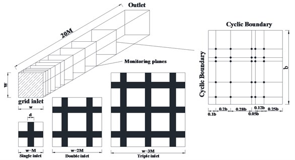
Table 1Boundary conditions

Location	Boundary conditions
Inlet flow	Velocity-inlet, $U =$ 1.92 m/s
Outlet	Outflow
Side wall	Symmetry
Top and bottom wall	Symmetry
Grid surface	Non slip wall

Table 2The details of cases

Case	Mesh density	Grid spacing $M$ (mm)	Bar width $b$ (mm)	Inlet period
1	32×32×800	40	10	Single
2	64×64×800	40	10	Double
3	96×96×800	40	10	Triple

2.3. Numerical validation

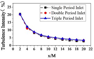
The turbulence intensity obtained by the present LES and the results of Tom Blackmore et al. [10] are presented in Fig. 2. The 10 monitoring points were set on the center line of the domain from 2 $< x / M <$ 20 downstream of the grid inlet, which is the same as the case of Tom Blackmore et al. It is shown that the turbulence intensity found by the current 3D LES aligns well with that obtained by Tom Blackmore et al. (2013).

The comparison results verify the accuracy of the current 3D LES works. The turbulence characteristics of three different grid inlets are studied with respect to the turbulence intensity, turbulence integral scale and lateral correlation of the fluctuating wind so as to investigate the domain requirements for implementing the grid-inlet technique.

Fig. 2Comparisons of turbulence intensity results obtained by current LES and results of Tom Blackmore et al. [10]

a) Single period inlet

b) Double period inlet

c) Triple period inlet

3. Results and discussions

3.1. Turbulence intensity and turbulence integral scale

As shown in Fig. 3, the results are compared with three different grid inlet periods to study the influence of domain sizes on turbulence intensity and the turbulence integral scale along the center line from 2 $< x / M <$ 20 (2 $x / M$ apart).

As shown in Fig. 3(a), the decay rate of turbulence intensity are unaffected by the domain sizes for three different grid inlet periods. However, as can be seen in Fig. 3(b), the integral scales of the three grids’ inlet flows are significantly different. The turbulence integral scale of the Single Inlet stabilizes at 0.2 $M$ . It is significantly smaller than the other two grids’ inlet flows because the size of the boundary is too small ( $w = M$ ), which limits the development of the turbulent vortices. The Double Inlet’s flow integral scale stabilizes at 0.4 $M$ . However, the Triple Inlet’s flow integral scale continues to increase and eventually stabilizes at 0.46 $M$ .

After the turbulence has been fully developed, the integral scales can be listed from largest to smallest as follows: Triple Inlet, Double Inlet, Single Inlet.

Fig. 3Influence of domain sizes on the turbulence intensity and integral length scale

a) Turbulence intensity (%)

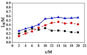
b) Integral length scale ( $L_{x} / M$ )

3.2. Fluctuating wind power spectrum

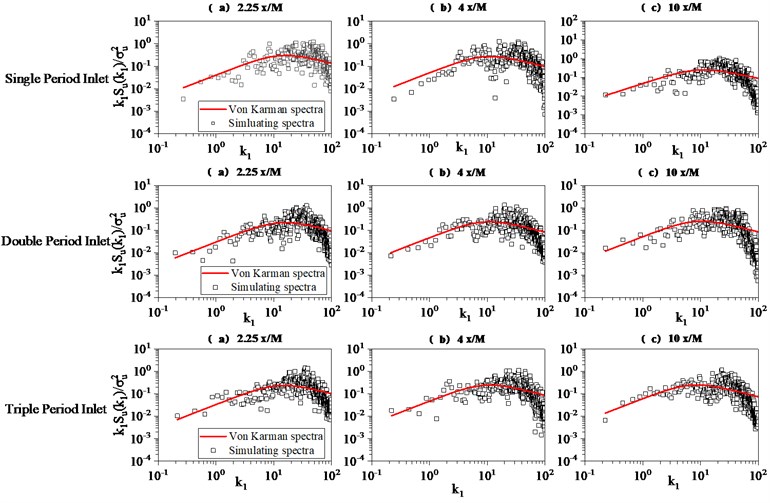
Normally, the turbulent flow generated by the grid basically satisfies the isotropic hypothesis. From the perspective of the wind spectrum, Roberts and Surry [11] found that the turbulent field generated by the grid could be accurately simulated by the von Kármán spectrum:

3

S_{u} (k_{1}) = \frac{4 σ_{u}^{2} L_{u}}{{[1 + 4 π^{2} {(1.339 L_{u})}^{2} k_{1}^{2}]}^{5 / 6}},

where, $k_{1} = n / U$ ( $n$ is frequency (Hz); $U$ is mean velocity); $L_{u}$ is longitudinal turbulence integral scale; $σ_{u}$ is standard deviation of longitudinal fluctuating velocity.

The results are compared with three different grid inlet periods to study the influence of domain sizes on the fluctuating wind power spectrum. Fig. 4 shows the power spectrum of the longitudinal fluctuating wind for three different grid inlet periods at 2.25 $x / M$ , 4 $x / M$ and 10 $x / M$ away from the grid inlet on the center line of the computing domain. The results show that the simulations of the longitudinal fluctuating wind spectra for the three different domain sizes align well with the von Kármán spectrum. It is proven that the grid-generated turbulence basically satisfies the isotropic hypothesis and is not affected by the domain sizes.

Fig. 4Effect of inlet grid period on the isotropic hypothesis

3.3. Lateral correlation of fluctuating wind

Normally, the correlation coefficient expressed by the time domain set average can be used to describe the correlation degree of two points of fluctuating wind speed in space (Eq. (4), Eq. (5)):

4

u (\overset{⃑}{x}, t) = [u_{1}, u_{2}, u_{3}],

where $u_{1}$ , $u_{2}$ , $u_{3}$ are the fluctuating wind speed in the $x$ , $y$ and $z$ directions, and are the function of place and time $(x, y, z; t)$ . For any two points in space, the cross-correlation function of the fluctuating components can be expressed as the second-order tensor matrix of 3×3:

5

R_{i j} (\overset{⃑}{r}, τ) = 〈u_{i} (\overset{⃑}{x}, t) u_{j} (\overset{⃑}{x} + \overset{⃑}{r}, t + τ)〉,

where, < > represents the ensemble average of two fluctuating components; $\overset{⃑}{r} = (r_{1}, r_{2}, r_{3})$ is the distance vector of two points in space ( $r_{1}$ , $r_{2}$ , $r_{3}$ is the distance along the $x$ , $y$ and $z$ axes).

In this paper, the lateral correlation of fluctuating wind is studied by arranging the transverse positions of monitoring points irregularly and in equal proportion, as shown in Fig. 2. Because the domain sizes of the three kinds of grid inlets are different, dimensionless processing is used for the transverse distance through $∆ y / b$ , where $b$ is the width of each computational domain. As can be seen from Fig. 5(a), the Double and Triple grids show basically the same changes in the lateral correlation of the longitudinal wind. The Triple Inlet changes more gently. However, the Single grid has a larger lateral correlation. As can be seen from Fig. 5(b), the three grids exhibit basically the same changes in the lateral correlation of vertical wind when $∆ y / b > 10$ . When $∆ y / b < 10$ , the Single grid has a significant lateral correlation of vertical wind because the computational domain of the Single grid is so small that the turbulence can not be totally developed.

Fig. 5Influence of domain sizes on the lateral correlation of fluctuating wind

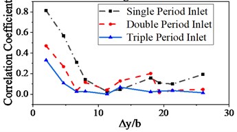
a) Longitudinal wind

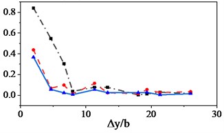
b) Vertical wind

4. Conclusions

In this paper, the author uses the new grid inlet technique to generate isotropic turbulence with higher intensity (up to 20 %). The main conclusions of this study are as followed:

1) The turbulence intensity decay rate is unaffected by the domain sizes.

2) The turbulence integral scale is proportional to the domain sizes, with a higher a steady value for larger domain size.

3) The gird-generated turbulence basically satisfies the isotropic hypothesis, not affected by domain size.

4) When lateral distance $∆ y / b < 10$ , the lateral correlation of fluctuating wind is inversely proportional to domain sizes; when lateral distance $∆ y / b > 10$ , the lateral correlation of three kinds of grids have basically the same change.

5) Through comparison and analysis, the triple inlet grid period (3 $M$ ×3 $M$ ) is the minimun domain size to make turbulence fully developed.

This study investigated the requirements of domain sizes for implementing the grid-inlet technique by studying the turbulence characteristics of three different grid inlets. By using the new grid inlet technique, the turbulence with different turbulence characteristics can be generated through deliberate selection of grid size and inlet length. The results of this paper could be helpful in the further application of the grid inlet technique.

References

Tabor G. R., Baba Ahmadi M.-H. Inlet conditions for large eddy simulation: a review. Computers and Fluids, Vol. 39, Issue 4, 2010, p. 553-567.

Publisher
Chung Yong Mann, Sung Hyung Jin Comparative study of inflow conditions for spatially evolving simulation. AIAA Journal, Vol. 35, Issue 2, 1997, p. 269-274.

Publisher
DeVillers E. The potential of Large EDDT Simulation for the Modeling of Wall Bounded Flows. Imperial College of Science, Technology and Medicine, 2006.

Search CrossRef
Carati Daniele, Ghosal Sandip, Moin Parviz On the representation of backscatter in dynamic localization models. Physics of Fluids, Vol. 7, Issue 3, 1995, p. 606-616.

Publisher
Wang Lian-Ping, Chen Shiyi, Brasseur James G. Examination of hypotheses in the Kolmogorov refined turbulence theory through high-resolution simulations. Part 2. Passive scalar field. Journal of Fluid Mechanics, Vol. 400, 1999, p. 163-197.

Publisher
Smirnov A., Shi S., Celik I. Random flow generation technique for large eddy simulations and particle-dynamics modeling. Journal of Fluids Engineering, Vol. 123, Issue 2, 2001, p. 359-371.

Publisher
Davidson L. Using isotropic synthetic fluctuations as inlet boundary conditions for unsteady simulations. Advances and Applications in Fluid Mechanics, Vol. 1, Issue 1, 2007, p. 1-35.

Search CrossRef
Fathali M., Klein M., Broeckhoven T., et al. Generation of turbulent inflow and initial conditions based on multi-correlated random fields. International Journal for Numerical Methods in Fluids, Vol. 57, Issue 1, 2008, p. 93-117.

Publisher
Nelkin M. Turbulence: An Introduction for Scientists and Engineers. Physics Today, Vol. 58, Issue 10, 2005, p. 80.

Publisher
Blackmore T., Batten W. M. J., Bahaj A. S. Inlet grid-generated turbulence for large-eddy simulations. International Journal of Computational Fluid Dynamics, Vol. 27, Issues 6-7, 2013, p. 307-315.

Publisher
Roberts J. B., Surry D. Coherence of grid generated turbulence. Journal of the Engineering Mechanics Division, Vol. 99, Issue 6, 1973, p. 1227-1245.

Publisher

Cited by

Wind Turbine Aerodynamics Modeling Using CFD Approaches

Galih Bangga

(2022)

About this article

Received

04 March 2020

Accepted

27 March 2020

Published

02 April 2020

SUBJECTS

Mathematical models in engineering

DOI

https://doi.org/10.21595/vp.2020.21370

Keywords

LES

gird Inlet technique

turbulence characteristics

CFD

Acknowledgements

This study was funded by the Natural Science Foundation of Chongqing, China, Grant No. cstc2018jscx-msyb1299, the Science and Technology Research Program of Chongqing Municipal Education Commission under the grant number KJZD-K201802501 and Graduate Scientific Research and Innovation Foundation of Chongqing under the grant number CYB17042.

This is an open access article distributed under the Creative Commons Attribution License, which permits unrestricted use, distribution, and reproduction in any medium, provided the original work is properly cited.

Previous article in issue Previous Next article in issue Next

Research article

2023 11 27

Investigation of the aerodynamic characteristics of single-box girders with different aspect ratios

Zhisheng Xue, Xiaowei Wang, Juncheng Zhou, Zhao Xiao, Xin Deng

Research article

2017 10 21

Numerical simulation analysis of large eddy simulation for T-tube based on solid-liquid two-phase abrasive flow

Jun Ye Li, Wen Qing Meng, Xiang Zang, Xin Ming Zhang

Research article

2017 09 30

Systematical research on the aerodynamic noise of the high-lift airfoil based on FW-H method

Cun Dong Tang, Zhi Ping Wang, Yu Zhou Sima

Research article

2017 06 30

Quality analysis of T-tube with solid-liquid two-phase abrasive flow polished

Junye Li, Lili Wei, Xinming Zhang, Jinglei Hu, Ningning Su

Z. Zhiwei, W. Bo, Z. Liangliang, W. Yuanqing, and H. Longxian, “Large-eddy simulations of the inlet grid-generated turbulence,” Vibroengineering PROCEDIA, Vol. 30, pp. 214–220, Apr. 2020, https://doi.org/10.21595/vp.2020.21370

Copy Extrica

Copied to clipboard!

TY  - JOUR
DO  - 10.21595/vp.2020.21370
UR  - https://doi.org/10.21595/vp.2020.21370
TI  - Large-eddy simulations of the inlet grid-generated turbulence
T2  - Vibroengineering PROCEDIA
AU  - Bo, Wu
AU  - Zhiwei, Zhang
AU  - Liangliang, Zhang
AU  - Yuanqing, Wang
AU  - Longxian, Huang
PY  - 2020
DA  - 2020/04/02
PB  - JVE International Ltd.
SP  - 214-220
VL  - 30
SN  - 2345-0533
SN  - 2538-8479
ER  - 

Copy Ris

Copied to clipboard!

@article{Bo_2020,
	doi = {10.21595/vp.2020.21370},
	url = {https://doi.org/10.21595/vp.2020.21370},
	year = 2020,
	month = {apr},
	publisher = {{JVE} International Ltd.},
	volume = {30},
	pages = {214--220},
	author = {Wu Bo and Zhang Zhiwei and Zhang Liangliang and Wang Yuanqing and Huang Longxian},
	title = {Large-eddy simulations of the inlet grid-generated turbulence},
	journal = {Vibroengineering {PROCEDIA}}
}

Copy Bibtex

Copied to clipboard!

[1]W. Bo, Z. Zhiwei, Z. Liangliang, W. Yuanqing, and H. Longxian, “Large-eddy simulations of the inlet grid-generated turbulence,” Vibroengineering PROCEDIA, vol. 30, pp. 214–220, Apr. 2020, doi: 10.21595/vp.2020.21370.

Copy IEEE

Copied to clipboard!

Bo, Wu, Zhang Zhiwei, Zhang Liangliang, Wang Yuanqing, and Huang Longxian. “Large-Eddy Simulations of the Inlet Grid-Generated Turbulence.” Vibroengineering PROCEDIA 30 (April 2, 2020): 214–20. https://doi.org/10.21595/vp.2020.21370.

Copy Chicago

Copied to clipboard!

Large-eddy simulations of the inlet grid-generated turbulence

Abstract

1. Introduction

2. Numerical model and basic methods

2.1. Governing equations and numerical algorithm

2.2. Computational domain, mesh, and boundary conditions

2.3. Numerical validation

3. Results and discussions

3.1. Turbulence intensity and turbulence integral scale

3.2. Fluctuating wind power spectrum

3.3. Lateral correlation of fluctuating wind

4. Conclusions

References

Cited by

About this article

Related Articles