Automatic decision making system with environmental and traffic data

1. Introduction

In last years, we see that switching to autonomous vehicles in vehicle technology is accelerating. Autonomous vehicles are vehicles that can sense surrounding environment and travel without any human intervention. Autonomous vehicles can sense the environment with technologies like radar, LIDAR, odometer and computer vision. When we look into history of autonomous vehicles, we see that first autonomous projects appear in 1980s. First prototype came to life with navlab and ALV projects that ran by Carnegie Mellon University. Followed by project Eureka Prometheus by Mercedes-Benz and Bundeswehr partnership at 1987. After these, lots of company manufactured many more and some of these vehicles could find a place in active traffic in some countries.

It is believed that in near future, autonomous vehicles cause an unprecedented change in economic, social and environmental areas of life. Based on these results, in this study, we aimed to build a software that can autonomously extract data related to factors of vehicle environment. In this study, we build three models that can carry out some predictions about vehicle environment in a certain domain with video footage from a vehicle centered camera as input. First model is an SVM that can detect vehicle positions on image. Second model fits a linear-parabolic function for right and left lane boundaries of the vehicle. Third model approximates a bird-view version of image and it could carry out a more realistic approximation of steer angle on bird-view image, rather than original.

Today’s autonomous vehicles use the locations of other vehicles in their environment to determine their routes. This is sufficient for the desired result, but it can be made even more effective with the information about where those vehicles are and where they may be. Therefore, the usage of object detection and classification plays an important role in that regard. The aim of object detection is to successfully detect and classify the objects, which are predefined, and to specify their position in an image.

The detection, thus classifications, of objects surrounding autonomous vehicles can be done by using the standard methods which are based on feature matching techniques using sets of pre-taught features. For low level object detection and recognition, techniques i.e. SIFT [1] and SURF [2] are utilized. For high level feature extraction techniques such as Haar Features [3] and HOG [4] are found to be more useful. They have shown good performances in the detection of Human [5-7] which is the most important feature in automatic decision-making system for self-driving vehicles [8, 9] or autonomous [10-13].

The development of autonomous vehicles will depend on the detection system design [14, 15] and processor speed [16, 17], which are high-tech products. In order to achieve this development, it is also important to support sensor production and logistically. These hardware features will be used more effectively with the software. In addition to security problems [18, 19], development of production capabilities in sensors and software, another problem to be solved is energy management [20].

Our study focuses on the development of software decision-making systems in automotive vehicle technology.

2. Method

In this section, the method used for the image segmentation for the application of the proposed clustering framework is discussed. In order to analyze image meaningfully with ease, image segmentation is performed. The division or partitioning of a digital image into several sub-regions with the aim to converting the image into a representation is called image segmentation. The recognition and thus classification of resultant pixel can be labelled as clustering a problem where each pixel represents a part of an object forming the original image.

The difference between pixels can be defined by many methods i.e. by using their brightness, color, texture, edge variations or their combinations. In this research, Histogram Over Gradient (HOG) is used to find similar cluster forming an image.

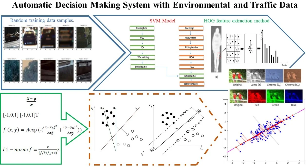
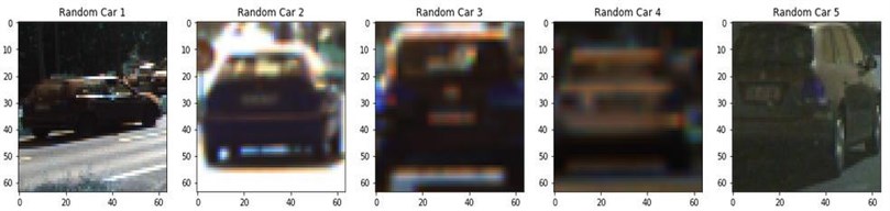
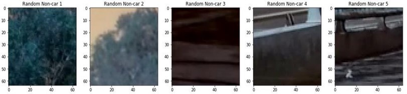
Like many systems that utilizes automatic decision making, machine learning techniques were used in this project, and positive and negative sample groups were needed for training. The sample data set was created by combining the GTI and the KITTI vehicle image databases (Fig. 1).

Fig. 1Random training data samples

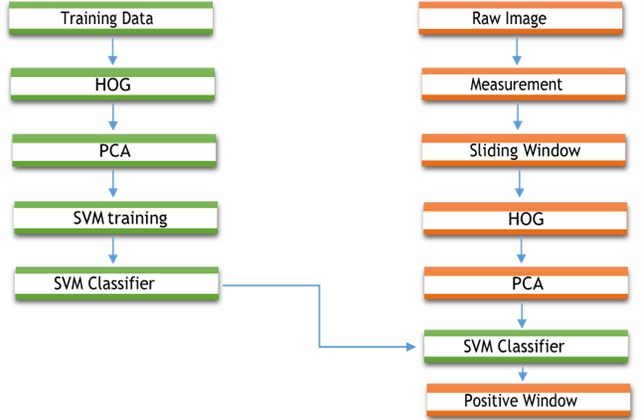
The data from the HOG algorithm was used in the training of the decision-making mechanism with the SVM (see 2.3.2) algorithm. The SVM model (see Fig. 2) obtained after training was subjected to standard normalization. PCA (see 2.3.3) algorithm was used as one of the ways to reduce transaction intensity. After the completion of training part, vehicle detection was performed in a 1280×720 pixel image array using the sliding window method.

In the future, it is planned to calculate the speeds of the detected vehicles and to apply the lane changing system with an appropriate lane detection system.

Fig. 2SVM model

2.1. Histogram of oriented gradients (HOG)

The basic idea behind the HOG algorithm is that the object found in any region of the view can be identified by color intensity variations (derivatives) or edge detection. The image is divided into small pieces called cells, and a vector histogram is generated containing the directions of the derivatives for the pixels in each cell. To increase the accuracy, cellular histograms can be normalized by assuming a relatively larger segment of the region (see Fig. 3). In addition, normalized results give better results in shadows and reflections.

There are a few features that positively distinguish the HOG algorithm from the others. Because the algorithm operates at the cellular level, it is unregistered against geometric and photometric changes except object orientation. That is, the performance of the observer is successful in almost every case where there is no major change in the overall appearance.

Fig. 3A demonstration of the HOG feature extraction method: a) the input image; b) gradient map with gradient strength and direction of a sub-block of the input image; c) accumulated gradient orientation; and d) histogram of oriented gradients [14]

$n$ the derivative calculation, the kernel that shows the most success in most applications is one-dimensional vector mask Eq. (1) and (2):

1

$\left[-\mathrm{1,0},1\right]\left[-\mathrm{1,0},1\right]T,$

2

$f\left(x,y\right)=A\mathrm{e}\mathrm{x}\mathrm{p}\left(-\left(\frac{{\left(x-x_0\right)}^2}{2{\sigma }_x^2}+\frac{{\left(y-y_0\right)}^2}{2{\sigma }_y^2}\right)\right).$

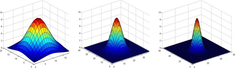
In addition, the Gaussian kernel (see Fig. 4) applied before the derivation calculation process provides a slight increase in performance in practice.

Fig. 4Gaussian kernel visualization

The derived image is divided into cells at the next step of the application. Each pixel in the cells uses a weighted game that specifies the direction of the derivative on the histogram divided by 0-180 or 0-360. The voting weight itself can be a derivative or a function of a derivative, but usually the derivative at Eq. (3):

3

$\frac{X-\mu }{\sigma }.$

The blocks are then typically formed into rectangular or circular blocks. Rectangular blocks are preferred in this project. Blocks can be on top of each other, so a cell can provide data to more than one block. The data passes through a separate normalization process after being collected in blocks. L1-norm is preferred for this application (see Eq. (4)):

4

$\mathrm{L}1\text{-}\mathrm{n}\mathrm{o}\mathrm{r}\mathrm{m}:f=\frac{v}{({‖\vartheta ‖}_1+e)}.$

2.2. Support vector machines (SVM)

The SVM core function is very similar to the logistic regression, that is to divide the data into groups, dividing a p-dimensional data group with a ($p-1$)-dimensional hyperplane. But the most important feature that differentiates the SVM from the logistic regression and puts it ahead of practice in performance is that SVM tries to maximize the gap between different data groups (see Fig. 5(a)). This approach offers a much more distinctive distinction between data groups.

Once collected, the histograms separated by the greatest difference from the others should be locally normed so that they do not affect the final result alone. It is better to use standard deviation instead of arithmetic average for normalization itself is the most accurate result.

SVM minimizes the error function shown below to ensure that we obtain the necessary parameters and obtain a hyperplane that separates the data into groups (see Fig. 5(b)).

However, with this method, points that are far from where it should be at hyperplanes can affect the end result. To avoid this, a one-dimensional Gaussian kernel centered on the hyperplane is used. Weights are obtained for each data point and the effect of distant points is reduced compared to the nearest point.

Fig. 5a) SVM convergence, b) maximum margin and support vectors

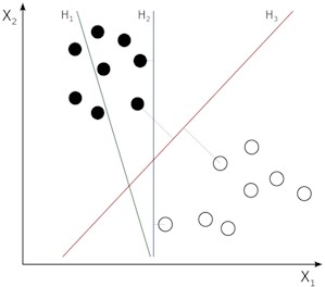
a)

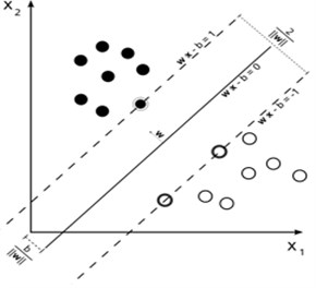
b)

2.3. Principal component analysis (PCA)

PCA can be thought of as fitting $n$-dimensional ellipsoid into data. Each axis length of ellipsoid represents a principal component. If an axis length of ellipsoid is short, the data point distribution along that axis is too small, and if the short axis is removed from the data we lose very little data (see Fig. 6(a)).

Fig. 6a) PCA of a multivariate Gaussian distribution, b) PCA implementation

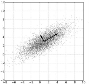
a)

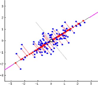
b)

Following the PCA implementation, the data points are reduced to projection onto the existing self-vectors (see Fig. 6(b)). In the end, variables that have almost no effect are removed from the data group.

In order to find the ellipsoid axis lengths, we first have to calculate the arithmetic mean of each variable from the data set. As a result of this process, the data group will be positioned around the origin. Then, the covariance matrix of the data is found, and the eigenvectors of the covariance matrix and the eigenvectors corresponding to the eigenvalues are computed. Then the eigen-vectors are normalized to be reduced by the unit vectors.

As a result, the data diversity that each eigen-vector represents can be calculated by dividing the corresponding eigen-value by the sum of all eigen-values.

2.4. Deep feedforward network

A different and more complex artificial neural network approach has also been dealt with because the optimization algorithm described at uses a small amount of function space that can be transformed if the data is used without pre-processing and the pre-processing takes a long time.

A neuron (unit/element) of an artificial neural network is basically composed of two functions. The functions should be selected as linear in the first and non-linear (activation) in the second. A neuron mathematically can be written as follows, where $h$ is the output value of the neuron, $g$ is the nonlinear function, $x$ is the input value of the neuron, $W$ is the matrix of the weight matrix and $b$ is the matrix of constants. The formula is seen at Eq. (5):

5

$h=g\left(W^{T}x+b\right).$

One of the most important features that distinguish artificial neural networks from classical machine learning methods is that the second part of neurons, that is, the activation parts, can be transformed into elements of a large function space as the model increases in depth. Without the activation function, the model is reduced to a series of linear functions, and the weight matrices of these inline linear functions can be written as a single matrix with the appropriate multiplication, indicating that the entire model can be reduced to a single linear combination without activation functions.

In real world applications, it is rarely possible for a given task to have only linear connections between input and output values, or a small number of nonlinear relations. Because of this and the constant increase in the power of data processing, deep learning methods and artificial neural networks are finding themselves in the spotlight day by day. And a deep learning model has also been added to this project, although results obtained cannot be labelled as successful.

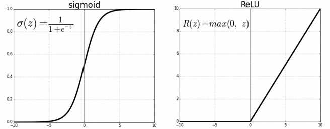
The choice of non-linear functions in the applications is the biggest factor affecting the learning speed and the overall performance of the model. The ReLU (rectified linear unit) function (see Fig. 7) was chosen as the activation function in the hidden layers of the model designed in this project and the sigmoid activation function was used because the output layer showed the desired Bernoulli distribution.

Fig. 7Sigmoid and ReLU functions

In order to optimize the model, forward propagation and back propagation algorithms should be performed. Forward propagation is the calculation of the output value and the loss function of the model according to the input values from the beginning to the end of the model at Eq. (6):

6

$L\left(y,\dot{y}\right)=-y\mathrm{l}\mathrm{o}\mathrm{g}{\dot{y}}^{\text{'}}-\left(1-y\right)\mathrm{l}\mathrm{o}\mathrm{g}\left(1-\dot{y}\right),$

as described above. “Cross-entropy loss” is used as the loss function.

The backpropagation algorithm is simply a derivation of the loss function with respect to all weight matrices. Contrary to forward propagation, back propagation is performed from the output units to the input units. Because the chain of calculus requires it.

After the derivative calculation, each element of the weight matrices is updated in proportion to its derivative at Eq. (7):

7

$W_{ij}=W_{ij}+\mathrm{}∆W_{ij},∆\mathrm{}{W}_{ij}=\mathrm{}-\eta \frac{\partial E}{\partial ∆\mathrm{}{W}_{ij}}.$

This process is performed one or more times at each pass over the data set. As a result, the extreme point of the loss function is determined.

3. Results

The general representation of the methods used up till now in this project has been made up to this division. The solutions to the following problems will be reviewed.

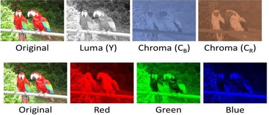
Firstly, SVM was trained with various color spaces in order to select the color space that is most compatible with the HOG algorithm and data set. 90 % of the data group for training and 10 % for the lead test were allocated. In the pioneer tests, the color space was “YCbCr” with accuracy between 94-97 %, which provides the highest accuracy (see Fig. 8). However, in the tests performed on the 1280×720-pixel image array, the actual power required for the real-time operation of the application was reached as the result of exceeding the capacity of the test device. In this phase, the PCA algorithm was included in the project. PCA was used in all channels of color space with 5292 variable numbers indexed to 3000. A natural increase in the training period and a 15-20 % decrease in the test duration were observed. However, despite the decrease in test time, vehicle detection was not even close to real-time. Processes performed at 3.1-3.4 s/frame prior to PCA could only reach 2.5-2.8 s/frame later. The SVM was abandoned for accuracy and the grayscale was selected as a color space with a range of 91-95 %. The data expressed in three different channels with the greyscale color space is reduced to a single intensity value. In 64×64 pixel images, the number of variables went down to 1764. It was then pulled to 1000 by applying PCA and processed at 1.15-1.35 s/frame. 5×5 to further reduce the time. According to Gaussian kernel, the entire data set was blurred prior to training and the SVM model was re-trained. An additional 5-10 % efficiency increase in processing speed was achieved without a statistically significant decrease in test accuracy. As a result, the processing speed has been increased to 1.0-1.3 s/frame.

Fig. 8Comparison of different color spaces

It is noted that in order to achieve the speed required for real-time study, the use of different architecture at processor level as well as by increasing process power the researches will be able to find solutions that will be much more economical. Different combinations of directions and cell numbers per block were tried to determine how the HOG algorithm’s parameters affected the test accuracy. The most successful results were obtained with 9 directions and 4 cell per block.

4. Discussion

One of the biggest challenges in the lane detection and tracking model is that the model is vulnerable to temporary or instantaneous changes in the image. Accordingly, while determining the area of interest for the next frame, the model’s resistance to changes was increased by adding a temporal filter application for the area of interest pixels. However, when the tests showed that the model resistance was not sufficient, the same application was applied to the central strip boundary orientations in addition to the temporal filter added to the pixels of interest and the changes that occurred more than 2 degrees per frame in a 25 fps image flow were ignored. In the tests performed after these two applications, it was found that the dynamic structure of the model was weakened, and it made more stable and consistent predictions. Another thing about the same model is that it is affected by color changes. Changes in the color of model road asphalt are affected by the shadows of trees and other vehicles (especially long and wide) on the side of the road. This effect affects the parabolic part of the approached part function rather than the linear part. In the model which makes the rotation angle estimation, a problem similar to the lane detection and tracking model is encountered. Considering the similarity of the techniques used by the models this can be said to be expected. The model is affected by road asphalt color changes and vehicle and tree shadows just like the other one. If the same solution is applied for this model, the error rate can be reduced in the dynamic regions of the road. Another aspect of this model is the increase in the error rate in the parts where the road slope changes.

The model uses the reverse perspective mapping method, which takes camera parameters as input. Although the position of the camera in space coordinates does not change, one of its parameters, lost point position, causes distortion in model estimation with the change of slope of the path. In order to prevent this situation, road slope changes can be estimated or determined by the image processing methods that we are interested in during our study, or with the help of various sensors that can be placed on the vehicle. After slope information, a separate model can be developed that can adapt to road slope changes for lost point estimation and the error rate can be greatly reduced.

5. Conclusions

The study is an autonomous driving support for improving artificial intelligence assisted driving behaviors and reducing human-related error parameters in general frame. This system consists of a decision-making algorithm based on game theory. The learned machine can be developed more rationally and reliably with logic and improved software and hardware support. With a communicative database to be created with this system, experience transfer of other tools can be provided and commercialized.