Design and analysis of experimental adaptive feedback system for active noise control (ANC) in a duct

1. Introduction

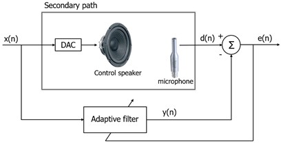
The physical implementation of the ANC system represents an electro-acoustic system where a control signal is generated to ensure destructive interference of the sound waves in the zone of interest [1]. The implementation of ANC systems is categorized into two types, feedback systems and feedforward systems (Fig. 1) [2]. In general, feedback systems are used to synthesize the control sound where it is necessary to perform active control of periodic single tone sounds with previously known frequency characteristics. These systems use a control sound sensor to determine the difference in the primary and control sound, which serves as feedback signal in the adaptive filter system. Unlike feedback systems, feedforward systems are applied to broadband (stochastic) sound and use two or more sound sensors, one to determine the characteristics of the primary unknown signal and others to determine the difference in sounds from the primary and the control speaker.

Fig. 1Fundamental setup of active noise control concept in a duct: a) feedback ANC system concept, b) feedforward ANC system concept

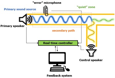
a)

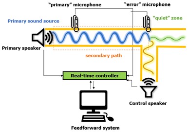
b)

To achieve a precise and stable active noise control system, a good choice of technical specifications of its components (sound source, sound sensor, as well as a processing unit for signal acquisition and processing) is of great importance. The sound sources should provide satisfactory dynamic range to be able to generate the frequencies of interest for noise control, the sound sensors should provide good sensitivity to the input measurement quantity, and the signal processor units should be able to reach good speed of response as well as fast convergence [3]. In addition to the technical requirements, another important aspect is the selection and correct modeling of the adaptive digital filter and the adaptive algorithm that directly affects the system characteristics.

The application of active noise control systems can be divided into applications for the reduction of unwanted sound in free space [4], sound reduction in cabin spaces [5], localized noise reduction (headphones) [6] and sound reduction in one-dimensional environment (HVAC systems) [7]. The noise that occurs in cooling or ventilation duct systems (HVAC systems) has a frequency composition with pronounced low frequencies, so passive methods are often insufficiently effective. In that direction, the state-of-the-art research in the literature indicates a favoring of the approach of active control of the sound in an acoustic environment in HVAC systems, which offers a quality application solution for the reduction of low-frequency noise in ducts. In the research paper [8], cancelling duct noises by using the ANC techniques is implemented. The authors describe the technique of using feedforward algorithm with feedback neutralization to realize ANC, where several kinds of ducts noises including tonal noises, sweep tonal signals, and white noise had been investigated. Experimental results show that the proposed ANC system can provide noise reduction of white noise up to 20 [dB]. In [9], the attenuation of sound propagation in an air-handling duct using robust and adaptive feedback active noise control strategies is investigated, with experimental results on active noise control in duct test bench. Paper [10] aims to design and analyze ANC performance in PVC duct experimentally for reducing periodic background noises, where a HMVSS method is proposed and developed in the feedback neutralization FxLMS algorithm. Within paper [11], a statistical approach to online secondary path modeling in active noise control is proposed. Adaptive filters are used to estimate the secondary path model and update it in real-time based on Bayesian analysis of input and output signals. Their work presents an improved approach in noise reduction systems which allows for improved sound quality. The authors in [12] focus on the impact of system uncertainties such as measurement noise and modeling errors, on the performance of the active noise control system. The authors present a stochastic analysis of feedback active noise control systems using the IMC approach and the FxLMS algorithm. Higher mode noise actively controlled in ducts can be seen in [13]. Active noise control is used in a duct using near field compensation and a ring of harmonic acoustic pneumatic sources. Ardekani et. al in [14] analyze the convergence behavior of real-time active noise control systems which can be used to reduce unwanted noise. The development of a new analysis approach provides a practical tool for assessing the convergence properties of these systems and for designing more effective control algorithms. A different approach for reduction of complexity of active noise control systems is developed in [15], by the introduction of a simplified version which makes it more accessible to a wider range of applications. This approach has been evaluated with simulated and experiment data and compared to traditional active noise control. On the other hand, a hybrid active and passive noise control approach is proposed in [16] for reducing noise in ventilation ducts which is considered a significant source of unwanted noise in buildings. The authors suggest that a combination of these two methods allows for greater noise cancelation than their individual use. Tahvilian et al. in [17] propose a narrowband ANC system that uses the FxLMS algorithm in noise reduction in ventilation ducts. In this context, the use of ANC as a sound source in ventilation ducts which might eliminate the need for traditional speakers is investigated in [18]. An active noise control system using Modal FxLMS algorithm is presented in [19] where it is used in noise reduction in a cylindrical cavity. The authors in [20] present the use of simulation models in real world noise reduction which might optimize the active noise control systems before their implementation in real-time settings, and in the same terms, the use of ANC for uncertain and time-varying disturbances is investigated by the researchers in [21]. The recent literature research in ANC systems implementation has proved that the use of two adaptive filter algorithms can significantly improve the overall adaptive filter performance, but also increase the computational cost of the system. Consequently, to solve this problem, the authors of [22] propose a new ANC structure based on FxNLMS and FxSLMS algorithms to reduce the computational cost of the ANC system.

The work presented in this paper focuses on the design and implementation of a system for active noise control of a one-dimensional acoustic environment, as a continuation of previous research given in [23]. The experimental setup for testing the active noise control system with previously chosen duct geometry, including the implemented hardware units is described. The system uses the feedback control approach, by integrating the FxLMS algorithm for neutralization of the secondary path in acoustic terms. The system is tested with tonal noises in frequency range from 100 [Hz] to 1 [kHz] and the results of the noise reduction are presented. A comparative analysis of literature review research papers correlated with the work of this paper is given in Table 1. As can be concluded, the ANC experiments dedicated on HVAC noise in ducts mainly focus on implementing complex feedforward ANC approaches with developing multiple adaptive algorithms, with target frequency for noise reduction above 200 [Hz]. Therefore, the main purpose of this work is to present a novel design methodology for developing an effective active noise control system with simplified and robust feedback approach, that is easy to implement, yet shows good potential. On the other hand, this system will provide its’ contribution to the literature gap noticed, by obtaining satisfying results in noise reduction focused on lower frequencies (from 100 [Hz] to 400 [Hz]) with systems with larger complexity.

2. Experimental setup of the active noise control system

In this work, within the framework of realization of the proposed system for active control of acoustic environment in a duct, the feedback control approach was applied. Feedback control systems imply the use of a single sound sensor for measuring the difference (“error” signal) between the characteristics of the primary sound and the control sound. The active control system consists of an acoustic duct, a primary loudspeaker for generating a single-tone signal, as well as a control loudspeaker for generating the control signal. To determine the characteristics of the control sound, it is necessary that the primary sound signal is measured by the reference sound sensor, which afterwards is sent to the signal processing controller in real time. Then, this information is processed in the software model, where the control design and modeling of the adaptive algorithms determine the characteristics of the control sound.

Fig. 2Experimental setup of the active noise control system of acoustic environment in a duct

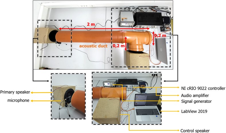
For the implementation of the active control system defined in these terms, a duct with a circular cross-section, with length of 2 [m] and diameter of 0.2 [m] was used. A side branch set on 90° for the control sound source was added. Two Visaton W 200-8 HiFi speakers were used to generate the sound signals. The control microphone is a PCB Piezotronics 130F20, which belongs to the class of TEDS sensors with an integrated EEPROM memory. To generate the primary sound signals, which in this case are periodic functions, an Agilent 335521A signal generator (function generator) and a Pioneer SA-508 audio amplifier were used. The entire experimental setup that was used for the active noise control system is presented in Fig. 2.

The implementation of the hardware control unit in ANC systems can be realized by using digital signal processors or FPGA modules. Digital signal processors have advantages due to the use of the C programming language, which makes them simpler for programming and design, but the FPGA module offers more serious advantages in the direction of achieving low power consumption and the possibility of parallel programming [24]. In this case, an NI 9234 analog signal acquisition card from National Instruments was used to acquire the audio signals from the microphone, while an NI 9263 analog signal generation card from National Instruments was used to generate the control signal from the control speaker. Both cards are added to the cRIO 9022 control module from National Instruments, which as a system has an integrated Real-Time (real-time) processing unit and FPGA chip, which enables high speeds and a high level of parallelism.

Fig. 3Setup of the Class 1 sound level meter Bruel and Kjaer

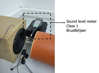
After installing the experimental postulation, in order to validate the sound reduction results in the acoustic zone of interest, a Class 1 sound meter from Bruel and Kjaer was also added to the system setup (Fig. 3). The instrument setup is chosen to be in the same position as the sound sensor to provide comparative sound intensity measurements, so the results for the $L_{AF}$ parameter for the sound level in [dB] before and after the application of the active control can be read appropriately.

3. Implementation of adaptive algorithms

Active noise control is a paradigmatic problem of adaptive signal processing, where a real-time control system generates a signal with the same frequency but opposite phase to the primary one, in order to achieve suspension of the unwanted sound (primary sound) in the desired zone. The anti-noise generated by the control source propagates through an electro-acoustic medium, called the secondary path, to reach the quiet point. The sound obtained in the “quiet zone” is called secondary sound. In this zone, primary sound and secondary sound combine with each other to form residual sound through the principle of destructive sound interference (Fig. (5)). By applying standard adaptive algorithms for active sound control, the residual sound is minimized by adjusting the control sound source (for example, the LMS algorithm minimizes the square of the residual noise).

An inevitable segment in the active sound control system that must be considered is the secondary path, which is an electro-acoustic signal channel that represents the return path of sound movement from the control sound source to the desired "quiet zone". From the point of view of classical control theory, the effect of the secondary path of the control system can be canceled if its inverse system is placed in front of the control sound source. This solution is trivial because the inverse system may be non-causal or unstable. An alternative solution is to filter the reference signal by estimating the secondary impulse response and then “feed” a standard adaptive algorithm from the filtered reference signal instead of the reference signal.

This solution leads to a series of adaptive algorithms known as Filtered-x adaptive algorithms. Due to the existence of the electro-acoustic secondary path between the control signal and the error sensor, the FxLMS algorithm is proposed in this system to neutralize the effect of the secondary path. In the FxLMS algorithm, an estimated secondary path model is required to maintain system stability. This model is typically obtained using either online or offline system identification techniques.

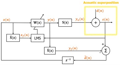
Fig. 4a) Block-diagram of the secondary path, b) Block-diagram of the feedback control by using FxLMS algorithm

a)

b)

In many applications, the actual model of determining the secondary path is time-variant, so it needs to be updated during the operation of the active control system. Otherwise, the system may become unstable, or its performance may decrease. In general, such algorithms can be categorized into two main classes: algorithms without adding noise and algorithms with adding noise. In noise-adding algorithms, typically white noise uncorrelated with the primary sound is dropped into the secondary path. An adaptive filter is then used to build the secondary path model by analyzing the effects of the added noise on the remaining sound. In this case, the full control system consists of two adaptive algorithms: secondary path modeling algorithm (Fig. 4(a)) and active control algorithm (Fig. 4(b)). The main disadvantage of such systems is the potential mutual interference between the two algorithms, which can lead to a low convergence rate of the secondary path modeling algorithm. Another disadvantage of noise-adding algorithms is that noise appears in the “quiet zone”, setting an upper limit on the maximum degree of sound reduction that can be achieved. Finally, noise-adding algorithms also require pre-initialization of the secondary path model because they are able to track only small changes in the secondary path.

The presence of transfer function of the secondary path $S\left(z\right)$ after the controller results in system lower stability of the LMS algorithm. This occurs due to the “error” signal, which is not correctly adjusted in time with the reference signal due to the presence of the secondary path $S\left(z\right)$. Therefore, an estimation of the secondary path $\widehat{S}\left(z\right)$ is suggested, in order to filter the reference signal $x\left(n\right)$ to update the weight coefficients of LMS algorithm, which results in FxLMS algorithm. On the block diagram in Fig. 4, FxLMS based system for active noise control is shown. The main idea of this system is to estimate the primary input sound signal $d\left(n\right)$ based on the “error” signal $e\left(n\right)$ and the output signal of the adaptive filter $y\left(n\right)$, where n is the time-index and the use of belated version of the estimated input signal $\overrightarrow{d}\left(n\right)$ as a reference signal $x\left(n\right)$ in the adaptive filter $W\left(z\right)$. Although, $S\left(z\right)=\widehat{S}\left(z\right)$, the physical path from the control source to the “error” sensor brings a time delay due to the time of sound propagation, so the synthetized reference signal is a belated version of the primary signal, i.e. $x\left(n\right)=d(n-\mathrm{\Delta })$, where $∆$ is approximated time delay of $S\left(z\right)$. In these terms, the system based on the interior model becomes adaptive predictor of $d\left(n\right)$ in order to minimize the residual sound $e\left(n\right)$ and its’ performance depends on the predictivity of the primary sound. It is known that $d\left(n\right)$ is not necessarily predictive in real conditions and therefore, a perfect sound cancellation is usually not obtainable. On the other hand, ideal estimation of the secondary path is also hard to achieve, due to the response of the secondary path that can be time-varying and can impact on the system efficiency.

On the block diagram given on Fig. 4, the yellow dashed line outlines the acoustic superposition. The interior reference signal $x\left(n\right)$ in the system can be expressed as given in Eq. (1):

where $y_f\left(n\right)={\overrightarrow{s}}^{-T}\overrightarrow{y}\left(n\right)$ is the estimated anti-signal obtained through filtering of the output signal $y\left(n\right)$. The output signal $y\left(n\right)$of the adaptive filter $W\left(z\right)$ that also denotes for the cancelling signal is given in Eq. (2):

where $x\left(n\right)$ is the reference signal vector and $w\left(n\right)={[w_0\left(n\right)w_1\left(n\right)\dots .w_{L-1\left(n\right)}]}^T$ is the adaptive weight vector. Here, $L$ denotes the length of the adaptive filter. The weight vector $w\left(n\right)$ updates based on the FxLMS algorithm (Eq. (3)):

where $\mu$ is the step-size of the convergence rate that gives the convergence speed and ${\overrightarrow{x}}_f\left(n\right)$ is the filtered vector of the reference signal. The “error” signal $e\left(n\right)$ is given with Eq. (4):

where $y_a\left(n\right)$ is the real anti-noise signal (Eq. (5)):

where $\overrightarrow{s}$ is a coefficient-vector with length $M$ that presents the impulse response of the real secondary path. In practical applications of active noise control, the secondary path model $\overrightarrow{s}$ is a short version of the real secondary path $s$, which means $n<m$. Therefore, the secondary path $S\left(z\right)$ is supposed to be known and its’ model $\widehat{S}\left(z\right)$ is obtained through offline modelling.

Taking into consideration this analysis, the active noise control system that applies FxLMS algorithm requires exact estimation of the secondary path model. Due to the restrictions of slower adaptation, the algorithm will converge between ±90° of phase error between $\widehat{S}\left(z\right)$ and $S\left(z\right)$. Therefore, the offline modelling of the secondary path uses secondary path identification with LMS algorithm and white noise as an excitement signal which is used $S\left(z\right)$ estimation in initial phase of system training when implementing the active noise control. Nevertheless, in applications that have a significant time-varying secondary path and require high performance, online modeling during operation of the active control system may be necessary.

4. LabView model for system control

The LabVIEW Real-time (LabVIEW RT) processor is intended for creating measurement and control systems in real time. On the other hand, cRIO 9022, in addition to the RT module, also contains an FPGA chip as a technology that enables the application of advanced algorithms for processing and management. The RT virtual instrument serves to maintain determinism such as, determining the number of boards that are read during transmission while preserving the data. Also, RT virtual instrument is used for visualization, post-processing, saving to files [25].

The user interface, that is, the front panel of the virtual instrument for determination of the secondary path modelling is presented on Fig. 5. Here, the input parameters for the LMS algorithm coefficient size and modeling time are set. The graphs show the amplitude-time input signal from the white noise generated by the control speaker, downstream to the primary speaker, then the measured signal reaching the microphone, and the difference in the two audio signals respectively. As mentioned, this stage is used at the beginning to determine the characteristics of the secondary track, while no control of the audio signal takes place.

Fig. 5User interface of secondary path determination in LabView

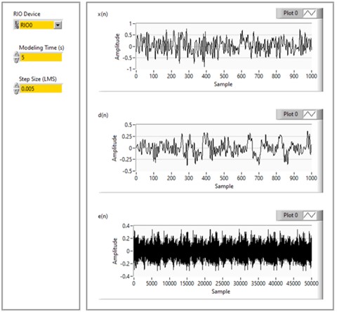
Fig. 6User interface of active noise control in LabView

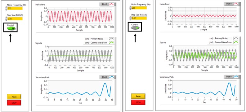
The front panel user interface given in Fig. 6 shows the RT virtual instrument for the phase where active control is implemented. As input parameters in this phase are the frequency of the signal, the size of the step of the FxLMS control algorithm and the on/off switch of the control speaker, i.e. activation and deactivation of the active control. Namely, the model for active control of the acoustic environment shown here, together with the experimental postulation, implements the feedback control, which implies that the sound signal generated by the primary speaker is a single-tone periodic signal with a known frequency. The step-size of the FxLMS control adaptive algorithm depends on the frequency of the primary sound signal, resulting in different active control performance of the system at different step sizes for different excitation frequencies. The step-size is tuned depending on the frequency of the sound signal generated by the primary speaker to ensure optimal operation of the system.

The first graphs in red in the two images (left and right) on Fig. 7 show the audio signal levels before (left) and after (right) activation of the active real-time control of the system for a selected representative frequency of 200 [Hz]. The second gray and green graphs respectively show the amplitude-time graphical representations of the primary and control sound signals. The third graphs below in blue show the coefficients of the secondary path determined by the LMS and FxLMS control adaptive algorithms.

5. Experimental results

The validity of performance of the designed experimental system, as well as the software model described, has been proven by testing 10 single-tone sounds with frequencies in the range from 100 to 1000 [Hz] (Fig. 7). Namely, sinusoidal signals were brought to the primary speaker in the experimental system by simulating them from the signal generator, through the audio amplifier. All input signals with the same amplitude are provided to the function generator of 80 [mVrms] and the same amplitude to the audio amplifier. It can be noted that the amplitude of the signals at different frequencies measured in the model in LabView is different, and this is due to the differences in the loudness of the signal at different frequencies. The graphs in Fig. 7 show a graphical visualization of the signals’ of all tested input frequencies (100 [Hz], 200 [Hz], 300 [Hz], 400 [Hz], 500 [Hz], 600 [Hz], 700 [Hz], 800 [Hz], 900 [Hz], 1000 [Hz]) amplitude in [V] levels in time [sps], before (left column) and after (right column) the application of the active control in the model, respectively. The sampling frequency chosen is 3 kHz (or 3000 [kS/s]), according to the frequency of the tested signals. The difference in the intensity of the amplitudes before and after the application of the control in the model can be clearly noticed, except for the 900 and 1000 [Hz] signals, where the noise reduction is evidently low when expressed in linear scale [V]. Therefore, the further analysis of the results required their conversion into [dB] which is shown in Fig. 8.

Fig. 7Amplitude [V] vs. samples per second (sps) graphs of sound reduction of 10 tested frequencies

a) 100 Hz

b) 100 Hz

c) 200 Hz

d) 200 Hz

e) 300 Hz

f) 300 Hz

g) 400 Hz

h) 400 Hz

i) 500 Hz

j) 500 Hz

k) 600 Hz

l) 600 Hz

m) 700 Hz

n) 700 Hz

o) 800 Hz

p) 800 Hz

r) 900 Hz

s) 900 Hz

t) 1000 Hz

q) 1000 Hz

In Fig. 8, the quantified sound reduction results for all frequencies tested are presented. The sound level in [dB] is measured using a Bruel&Kjaer Class 1 measuring instrument. It is expressed as L_AF parameter, which represents the maximum level with an A-weighted frequency curve and F velocity measurement characteristic, presented in [dB]. From the results shown in Fig. 8, can be concluded that the largest and most significant reduction is observed at frequencies of 200 Hz, 300 [Hz] and 400 [Hz], while at higher frequencies above 400 [Hz], the reduction in the sound level are isller.

Furthermore, additionally to the influence of the sound level reduction, can be noticed that the coefficients of the FxLMS adaptive algorithm show a significant influence on the convergence speed of the weighting coefficients and the stability of the system. The effects of the FxLMS algorithm have shown strong implications on system performance. Instead of destructive wave interference, constructive interference was observed due to incorrect achievement of the anti-phase control signal, which results in amplifying the noise, rather than reducing it.

Fig. 8Comparison of the sound level in [dB] before and after active noise control implementation

The conducted tests of the experimental system at different frequencies lead to a conclusion that the set values for the coefficient of the FxLMS adaptive algorithm have the greatest influence on the reduction of the sound volume level at all frequencies. The optimal results for the greatest volume reduction were obtained by tuning the coefficients of the algorithm manually. In Fig. 9, the sound reduction results achieved for all frequencies expressed in percentage [%] are shown. The values of the coefficients of the FxLMS algorithm for which these reductions were achieved are also given in Fig. 9.

From the results, it can be noted that the greatest reduction is achieved at a frequency of 200 [Hz] which is 17 % or 14 [dB]. A significant sound reduction was achieved at both 300 [Hz] and 400 [Hz] which is 12 %, i.e. 10 [dB] in both cases. At all frequencies above 400 [Hz], even with variations of the coefficient of the FxLMS algorithm, the maximum reductions achieved are in the range of 1 % to 3 %.

Fig. 9Reduction (in %) in the sound level [dB] of all 10 tested frequencies in dependence of the FxLMS coefficients

6. Future work

Considering the previously discussed challenges and opportunities of the developed active noise control system, the authors suggest experimental tests on HVAC duct with different characteristics. In these terms, it is proposed to provide experimental results of a duct with a different material (rubber, stainless steel, silicone, neoprene-dipped polyester fabric etc.) and different geometry, as well as side branch number and location. Also, the effect of source location and duct termination on acoustic power flow attenuation is an important aspect that needs to be considered and explored furthermore, to obtain better insights into the system applicability.

Active sound control applied to a spatially extended region is a challenging field of research aimed at creating a wider “quiet zone” in three-dimensional (3D) spaces. Undoubtedly, the creation of “quiet zones” or “quiet spaces” in people’s everyday life using not very expensive, applicable, and simple to implement active sound control systems is more than beneficial and desirable. These sophisticated solutions overcome the limitations of the simpler active control systems described above [26]-[29].

Fig. 10Proposed system for active noise control in three-dimensional space

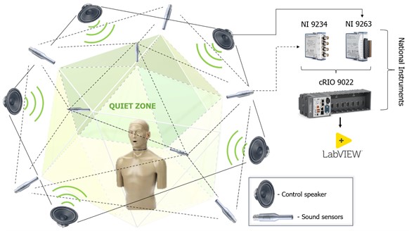
In this context, the authors propose creating a three-dimensional active noise control system, such that the hardware components used for the realization of the experimental model of an active system in a one-dimensional space can be applied again, with the addition of the number of sensor and control units (Fig. 10). Namely, the main component of the system can be the cRIO 9022 reconfigurable unit from National Instruments, which is an FPGA-based input-output module for working with real-time signals. Furthermore, NI 9234 analog signal acquisition module and NI 9263 analog signal generation module can be used again to add to the cRIO 9022 chassis. In addition, it is recommended that the already existing system be upgraded in the direction of enabling it to reduce a wide range of noise sources.

7. Conclusions

In this paper, an experimental design and implementation of simplified adaptive feedback system active noise control is presented. During the implementation of the active control system, the concept of neutralization of the secondary path is applied, which inevitably occurs due to the return acoustic energy from the secondary source to the sound sensor and can degrade and destabilize the power of the system. The validity and functionality of the proposed system is shown by conducted experimental tests for single-tone noise control. It is shown that the parameterization of the step size of the FxLMS adaptive algorithm greatly affects the optimal operation of the system, and with its correct leveling, neutralization of the secondary return path can be optimally achieved. This system is advantageous in computational load and ease of implementation which contributes to the development and application practice of ANC systems in terms of creating possibilities for a simplified feedback approach to develop an effective system. Although only a certain level of suspension of the acoustic environment can be obtained in practical terms, this approach proposes a robust methodology for the control of the acoustic environment as a solution that is easy to implement in real-time applications. Within the experimental results discussion it is perceived that the system shows great efficiency at lower frequencies in the range from 200 to 400 [Hz], where a reduction in sound intensity of up to a maximum of 17 % is achieved at 200 [Hz]. Compared to the literature reviewed, the noise reduction achieved on lower frequencies with such simplified and robust approach, suggests novelty in the proposed work.

On the other hand, two limitations in the implementation of the proposed system for active control of the acoustic environment can be noticed. The first refers to the fact that the system can provide control of the acoustic environment only for known primary single-tone signal. In order to overcome this disadvantage, a simplified feedforward system with multiple microphone units might potentially be developed and tested. The second limitation is the physical limitation of the zone in which the system can provide sound reduction. This is because only certain level noise attenuation can be obtained in practical simplified feedback ANC systems and the error signal always contains some portion of the primary noise. Also, the estimation of secondary path may be imperfect which results in the quality of reference signals in the simplified feedback ANC systems.