Abstract
A new simple well-behaved definition of the fractional derivative termed as conformable fractional derivative and introducing a geometrical approach of fractional derivatives, non-integral order initial value problems are an attempt to solve in this article. Based on the geometrical interpretation of the fractional derivatives, the solution curve is approximated numerically. Two special phenomena are employed for concave upward and downward curves. In order to obtain the solution of fractional order differential equation (FDE) with the integer-order initial condition, some new criteria on fractional derivatives are proposed.
1. Introduction
The impact of this fractional calculus in both pure and applied branches of science and engineering started to increase substantially during the last two decades apparently. Differential equations governing most of the physical system, evade closed-form solutions and thereby necessitating the adoption of numerical methods to arrive at the desired solutions of the equations. Moreover, in many practical situations, some of the coefficients or functions in the differential equation may be non-linear or are presented as a set of discrete data, and then, numerical methods become inevitable for obtaining solutions.
Since the last decade, fractional-order differential equations have gained considerably more attention due to their applications in many engineering and scientific disciplines. As the mathematical models for the systems and processes, the fractional differential equation has been successfully applied in various fields of physics and engineering such as biophysics, bioengineering, quantum mechanics, finance, control theory, image and signal processing. A rather detailed account of diverse recent theoretical advances and applications of fractional calculus in the various fields can be found in the books of Sabatier et al. [14], Hilfer [6] and Atanackovic et al. [1]. Works such as [2, 3, 7, 8, 11, 15, 16, 22-29] and the monographs [4, 13] analyzed qualitative and quantitative aspects of the solution of the fractional-order differential equation. The methods employed in the aforementioned literature include the sequential technique of successive approximation as well as the classical fixed-point approaches of Banach and Schauder. Othman et al. [20] studied the effect of hydrostatic initial stress and gravity on a fiber-reinforced thermoelastic medium with a fractional derivative heat transfer. The effect of hydrostatic initial stress on the plane waves in a fiber-reinforced magneto-thermoelastic medium with fractional derivative heat transfer was explained by Sarkar et al. [21].
In the sequel, we would confine our attention to developing an algorithm for solving the initial-value problem, namely:
Eq. (1) may be viewed as a curve in the -plane, at each point on the curve the value of its -order derivative is given in terms of and , however, refers to a particular curve that passes through a given point .
In an endeavour to incorporate the curvature of the curve to arrive at an approximate numerical solution of the initial-value problem (1); one tries to explore the possibility of alternative approaches. This leads to the following two types of procedures:
(i) Semi-analytical approach based on the power series expansion (see Refs. [5, 11, 15, 17]).
(ii) Numerical approach applying the geometrical interpretation of fractional derivatives. A new geometrical approach to obtain an approximate solution of FDEs, subject to integer-order initial conditions which are significant to describe most of the physical phenomena, is the main course of study of this paper.
2. Fractional Taylor series
An extensive introduction to the use and meaning of fractional derivatives in physical and biological systems can be found in the article Metzler and Klafter [9]. The fractional Taylor series is a generalization of the Taylor series of fractional derivatives. The fractional Taylor series at the point is defined by Odibat and Shawagfeh [10]:
where is the gamma Function, and is the Caputo fractional derivative of order with base point , which is defined by:
where is the usual first derivative, and the notation in Eq. (2) indicates the limit as we approach from the right. Note that there are other definitions of fractional derivatives, but the fractional Taylor series is valid for the Caputo form. The main distinguishing feature of the Caputo fractional derivative is that, analogous to integer order derivatives, the Caputo fractional derivative of a constant is zero. This property is very critical for a fractional Taylor series. It is also a notable fact that the third term of Eq. (2) involves the order fractional derivative of fractional derivative, which is not identical to the order fractional derivative.
To ensure this fact we consider the function:
where
Now the order derivative of Eq. (4) is a constant when , and the fractional derivative of that constant is zero. Then the coefficients of the fractional Taylor series can be found in the usual manner, by repeated fractional differentiations. The traditional integer-order Taylor series can be recovered from Eq. (2) when , applying the well-known property of the Gamma function .
The fractional Taylor series gives an extremely good estimation of non-integer power-law functions. We now adopt Eq. (4) for a non-linear power-law function, to illustrate this behaviour.
The traditional integer-order Taylor series approximation for Eq. (4) with , expanded about and truncated at the second-order term, is:
If and , Eq. (5) becomes:
Hence, the second-order Taylor series approximation is exact for because the order of nonlinearity of the function matches the order of the Taylor series approximation. If , a third-order Taylor series would provide an exact approximation.
However, if is a non-integer real number, no finite integer order Taylor series can give an exact match between the value of the function and its Taylor series approximation.
Now let us examine the fractional Taylor series approximation of Eq. (4), when is some real number. The Caputo fractional differentiation of Eq. (3) is:
Thus, first-order fractional Taylor series for (4) expanded about is exact when the first term is For the second term, use Eq. (7) along with the fact that the Caputo fractional derivative of the constant is zero to write:
Then for any we have (since the exponent so the term for any ):
Then of course the limit is:
Thus, the second term of fractional Taylor series is given by:
Here we have used and Since is a constant, the remaining higher order Caputo derivatives are all zero. Therefore, the two-term fractional Taylor series approximation is exact:
This is a very significant result. It proves that if we match the order of the fractional Taylor series approximation to the exponent in the power-law function, then the two-term fractional Taylor series approximation to that function is exact.
3. Modified Riemann-Liouville fractional derivative
In this section, we illustrate the fractional derivatives based on fractional differences which are slightly different from the classical Riemann-Liouville framework. The fractional calculus so obtained is quite parallel to the classical calculus, and it involves non-commutative derivatives, which seems to be quite consistent with non-commutative geometry. The purpose herein is to contribute some new results to this approach.
3.1. Fractional derivatives via fractional differences
Definition 1. (Fractional right derivative): Let be a continuous (not necessarily differentiable) function and let denotes the constant discretization span. The forward difference operator is defined by:
the fractional difference of order , from the right, of is defined by the expression:
and the corresponding fractional derivative on the right is given by:
Definition 2. (Fractional left derivative): The left hand (or backward) fractional difference of the function of order , is defined as:
and its fractional derivative on the left is given by:
These are local definitions as compared with the standard integral approach. These are very close to the standard definitions of derivative and as a direct result, the -order derivative of a constant is zero.
When to shorten in writing we shall set . Here we are fully in the Leibnitz framework, i.e., to say both and denote the finite increments.
3.2. Some important properties
Here we can mention few important properties of the aforementioned fractional derivative:
(1) The fractional derivative, as so defined, is not commutative. Clearly one has:
The equality holds if
(2) Let be a continuous function such that has fractional derivative of , where is any integer and , then:
(3) Let us consider the compound function . Assume that is -differentiable with respect to and is differentiable with respect to then:
(4) Assume that both as well as are -differentiable with respect to and respectively, then:
(5) One can extent the aforementioned fractional derivatives for negative order also i.e. of order , can be expressed in the following integral form:
For one can set:
The difference between Eqs. (22) and (23) is that the second one involves the constant whereas the first equation does not. We shall refer to this fractional derivative as the modified Riemann-Liouville derivative.
Proof. proofs of the properties (1)-(4) are left for the readers. For (5); take Laplace to transform with respect to x in both sides of the Eq. (23) and denoting yields:
Now according to the Eq. (15) (in definition 1):
Therefore, from Eq. (15) we get:
Hence the proof.
3.3. Fractional Taylor series with Mittag-Leffler function
Let us consider the continuous function , has a fractional derivative of order , for any positive integer and , , then the following relation holds:
where ( ( times), is the derivative of order ( times) of , and with the relation:
The definition of forwarding difference operator, given by the Eq. (13) and from the Eq. (14) one can show that the forward operator satisfies the following fractional differential equation:
and the solution of this equation is
Therefore, the series can be expressed in the following manner:
In which is the differential operator with respect to , and is the Mittag-Laffler function given by:
This fractional Taylor’s series does not hold with the standard Riemann-Liouville derivatives, and it applies to non-differentiable functions only. In addition, it is different from Osler’s series of fractional order [12].
4. The concept of approximation
In this section, we attempt to prove a special nature of the straight “line” (or tangent line) drawn at a point to the curve taking different order fractional derivatives as its slope at that point. To do that, firstly we demonstrate few important properties as follows:
Theorem 1. For any two real numbers and , or accordingly is a concave upward or concave downward function.
Proof. From the definition 1, for any real number :
where
Now it is clear that, if is a non-decreasing function then is also non-decreasing for all values for
Therefore:
Since, and , then for a concave upward function for all positive real values of
Thus, if is a concave upward function, for any two real numbers and , .
With the similar arguments, it can be prove that for a concave downward function , , where
Hence the Proof.
Therefore, in order to estimate the curve, for a concave upward function, the “lines” (or tangent lines) with the highest order fractional derivative where to the curve at the point will be a more appropriate one.
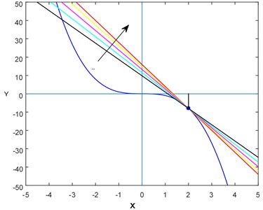
Whilst, for a concave downward curve, the “line” (or tangent) at a point having the slope with the lowest order fractional derivative where at that point to the curve would have been more suitable than the conventional tangent line.
5. Graphical illustration
Here we illustrate the nature of the tangent lines with different fractional-order derivatives where , which is taken as the slope of the line, for concave upward and downward curves. For this purpose, we have considered two simple polynomials (see Fig. 1 and Fig. 2).
Let be an approximation in the interval . Expanding about the point , we have:
where is the order derivative of at and
Fig. 1Various “lines” (or tangent lines) with different slopes for f(x)=x3
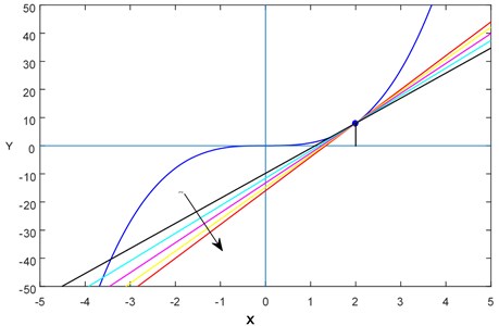
Fig. 2Various “lines” (or tangent lines) with different slopes for f(x)=-x3
Replace by in Eq. (35) we obtain:
Assuming the variation of is negligible in the truncation error can be put as .
Hence, to determine the function , which will be the solution of the initial value problem Eq. (1), may apply the following algorithm:
where is a constant to be chosen in such a way that or accordingly the curve is concave upward or downward i.e., or at .
6. Convergence criteria
A method is convergent if, for every ODE with a Lipschitz function and every fixed , with , it holds that:
Global error: and
Local error: where
Therefore, local error definition implies the residual:
Now comparing with the Taylor series expansion Eq. (28), the local error for this proposed method is .
Thus, the global error recursion is given by:
Take norms and use Lipschitz condition:
Lemma. If be a sequence of non-negative numbers satisfying , , , for , then , .
Proof. Standard result of sequence of real nos.
Theorem 2. Prove that the global error as approaches to zero.
Proof. Assuming that the function is sufficiently differentiable, given and a fixed , let us consider .
Applying the lemma to global error recursion, we get:
with:
Since:
We have, for :
Therefore:
which proves the convergence as:
Hence, the iteration converges invariably in keeping with expectation.
7. Applications
In order to assess the applicability of the proposed method, we have considered a number of fractional differential equations with initial conditions. The iteration procedure is carried out through computer simulation (MatLab 2015a) with a moderate value of the step length.
For the computational purpose we consider the following fractional order initial value problems.
Example 1. (Example – 4.1 [18]):
Example 2. (Example – 4.3 [18]) with :
Example 3. (Eigen value problem: example – 5.4 [19]):
Fig. 3Comparison of solutions between the analytical result and present analysis (Ex. 1)
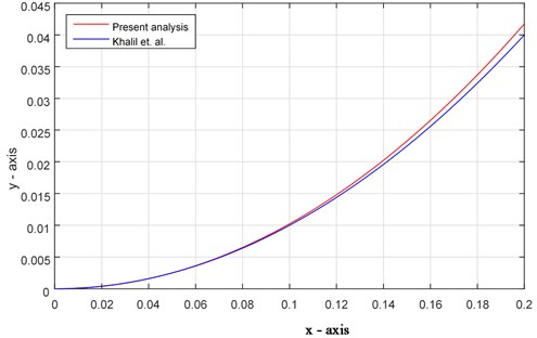
For numerical computation, in all of the above examples, we consider 0.001, 0.125 and 1. The analytical solutions for the considered initial value problems (IVPs) are presented in Table 1 (for details see Refs. [18, 19]). Those results are compared with the approximate solutions obtained by using the proposed method. It has been observed that the present approximations (by using the iteration scheme Eq. (37)) are in high agreement with the results obtained by [18]. Figs. 3-5 represent the solution curves of the IVPs Eqs. (48)-(50) by using the present analysis and analytical results. It has also been noticed that this newly adopted method is identical with the analytical solutions up to two decimal places.
Fig. 4Comparison of solutions between the analytical result and present analysis (Ex. 2)
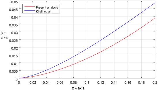
Fig. 5Comparison of solutions between the analytical result and present analysis (Ex. 3)
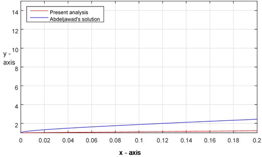
Table 1Analytical solutions of the IBPs
Example | IVP | Solution |
Ex. 1 | ||
Ex. 2 | ||
Ex. 3 |
8. Conclusions
With the help of the geometrical interpretation of fractional order derivatives for different values of the parameter at a fixed point on a curve, in this paper, we developed a new numerical iterative method that can give an approximate solution curve of the fractional initial value problems. Here we use two different values of fractional derivatives to approximate the solution curve for the concave and convex parts. Purely depending upon geometrical interpretation, this type of works have not yet been reported on a fractional differential equation.
During the decade, it has been established that several biological and physical aspects could be encompassed in the framework of a suitable fractional differential equation. We assert that the approach to the fractional calculus via fractional difference in combination with fractional Taylor’s series provides a method of approximation of the solution curve for IVPs in Leibniz’s sense. The proposed method could be fairly competent in this kind of problems.
References
-
T. M. Atanackovic, S. Pilipovic, B. Stankovic, and D. Zorica, Fractional Calculus with Application in Mechanics. London: Wiley, 2014.
-
K. Diethelm and N. J. Ford, “Analysis of fractional differential equations,” Journal of Mathematical Analysis and Applications, Vol. 265, No. 2, pp. 229–248, Jan. 2002, https://doi.org/10.1006/jmaa.2000.7194
-
K. Diethelm and N. J. Ford, “Multi-order fractional differential equations and their numerical solution,” Applied Mathematics and Computation, Vol. 154, No. 3, pp. 621–640, Jul. 2004, https://doi.org/10.1016/s0096-3003(03)00739-2
-
K. Diethelm, The Analysis of Fractional Differential Equations. Heidelberg: Springer, 2010.
-
A. El-Ajou, O. Arqub, Z. Zhour, and S. Momani, “New Results on Fractional Power Series: Theories and Applications,” Entropy, Vol. 15, No. 12, pp. 5305–5323, Dec. 2013, https://doi.org/10.3390/e15125305
-
R. Hilfer, Application of Fractional Calculus to Physics. Singapore: World Scientific, 2000.
-
V. Lakshmikantham and A. S. Vatsala, “Basic theory of fractional differential equations,” Nonlinear Analysis: Theory, Methods and Applications, Vol. 69, No. 8, pp. 2677–2682, Oct. 2008, https://doi.org/10.1016/j.na.2007.08.042
-
V. Lakshmikantham and A. S. Vatsala, “General uniqueness and monotone iterative technique for fractional differential equations,” Applied Mathematics Letters, Vol. 21, No. 8, pp. 828–834, Aug. 2008, https://doi.org/10.1016/j.aml.2007.09.006
-
R. Metzler and J. Klafter, “The restaurant at the end of the random walk: recent developments in the description of anomalous transport by fractional dynamics,” Journal of Physics A: Mathematical and General, Vol. 37, No. 31, pp. R161–R208, Aug. 2004, https://doi.org/10.1088/0305-4470/37/31/r01
-
Z. M. Odibat and N. T. Shawagfeh, “Generalized Taylor’s formula,” Applied Mathematics and Computation, Vol. 186, No. 1, pp. 286–293, Mar. 2007, https://doi.org/10.1016/j.amc.2006.07.102
-
Z. Odibat, S. Momani, and V. S. Erturk, “Generalized differential transform method: Application to differential equations of fractional order,” Applied Mathematics and Computation, Vol. 197, No. 2, pp. 467–477, Apr. 2008, https://doi.org/10.1016/j.amc.2007.07.068
-
T. J. Osler, “Taylor’s series generalized for fractional derivatives and applications,” SIAM Journal on Mathematical Analysis, Vol. 2, No. 1, pp. 37–48, Feb. 1971, https://doi.org/10.1137/0502004
-
Igor Podlubny, Fractional differential equations: an introduction to fractional derivatives, fractional differential equations, to methods of their solution and some of their applications. San Diego: Academic Press, 1999.
-
J. Sabatier, O. P. Agrawal, and J. A. Tenreiro Machado, Advances in Fractional Calculus.Theoretical Developments and Applications in Physics and Engineering. Dordrecht: Springer, 2007.
-
C. C. Tisdell, “On the application of sequential and fixed-point methods to fractional differential equations of arbitrary order,” Journal of Integral Equations and Applications, Vol. 24, No. 2, pp. 283–319, Jun. 2012, https://doi.org/10.1216/jie-2012-24-2-283
-
C. C. Tisdell, “Solutions to fractional differential equations that extend,” Journal of Classical Analysis, Vol. 5, No. 2, pp. 129–136, 2014, https://doi.org/10.7153/jca-05-11
-
X.-F. Zhou, F. Yang, and W. Jiang, “Analytic study on linear neutral fractional differential equations,” Applied Mathematics and Computation, Vol. 257, pp. 295–307, Apr. 2015, https://doi.org/10.1016/j.amc.2014.12.056
-
R. Khalil, M. Al Horani, A. Yousef, and M. Sababheh, “A new definition of fractional derivative,” Journal of Computational and Applied Mathematics, Vol. 264, pp. 65–70, Jul. 2014, https://doi.org/10.1016/j.cam.2014.01.002
-
T. Abdeljawad, “On conformable fractional calculus,” Journal of Computational and Applied Mathematics, Vol. 279, pp. 57–66, May 2015, https://doi.org/10.1016/j.cam.2014.10.016
-
M. Ibrahim Othman, S. M. Said, and N. Sarker, “Effect of hydrostatic initial stress on a fiber-reinforced thermoelastic medium with fractional derivative heat transfer,” Multidiscipline Modeling in Materials and Structures, Vol. 9, No. 3, pp. 410–426, Sep. 2013, https://doi.org/10.1108/mmms-11-2012-0026
-
N. Sarkar, S. Y. Atwa, and M. I. A. Othman, “The Effect of Hydrostatic Initial Stress on the Plane Waves in a Fiber-Reinforced Magneto-Thermoelastic Medium with Fractional Derivative Heat Transfer,” International Applied Mechanics, Vol. 52, No. 2, pp. 203–216, Mar. 2016, https://doi.org/10.1007/s10778-016-0748-4
-
O. Brandibur and E. Kaslik, “Stability analysis of multi-term fractional-differential equations with three fractional derivatives,” Journal of Mathematical Analysis and Applications, Vol. 495, No. 2, p. 124751, Mar. 2021, https://doi.org/10.1016/j.jmaa.2020.124751
-
N. D. Cong, H. T. Tuan, and H. Trinh, “On asymptotic properties of solutions to fractional differential equations,” Journal of Mathematical Analysis and Applications, Vol. 484, No. 2, p. 123759, Apr. 2020, https://doi.org/10.1016/j.jmaa.2019.123759
-
F. Alzahrani and I. A. Abbas, “Generalized Thermoelastic Interactions in a Poroelastic Material Without Energy Dissipations,” International Journal of Thermophysics, Vol. 41, No. 7, Jul. 2020, https://doi.org/10.1007/s10765-020-02673-0
-
T. Saeed, I. Abbas, and M. Marin, “A GL Model on Thermo-Elastic Interaction in a Poroelastic Material Using Finite Element Method,” Symmetry, Vol. 12, No. 3, p. 488, Mar. 2020, https://doi.org/10.3390/sym12030488
-
I. Abbas, “Natural frequencies of a poroelastic hollow cylinder,” Acta Mechanica, Vol. 186, No. 1-4, pp. 229–237, Oct. 2006, https://doi.org/10.1007/s00707-006-0314-y
-
A. M. El-Naggar, Z. Kishka, A. M. Abd-Alla, I. A. Abbas, S. M. Abo-Dahab, and M. Elsagheer, “On the Initial Stress, Magnetic Field, Voids and Rotation Effects on Plane Waves in Generalized Thermoelasticity,” Journal of Computational and Theoretical Nanoscience, Vol. 10, No. 6, pp. 1408–1417, Jun. 2013, https://doi.org/10.1166/jctn.2013.2862
-
G. Palani and I. A. Abbas, “Free Convection MHD Flow with Thermal Radiation from an Impulsively-Started Vertical Plate,” Nonlinear Analysis: Modelling and Control, Vol. 14, No. 1, pp. 73–84, Jan. 2009, https://doi.org/10.15388/na.2009.14.1.14531
-
R. Kumar and I. Abbas, “Deformation Due to Thermal Source in Micropolar Thermoelastic Media with Thermal and Conductive Temperatures,” Journal of Computational and Theoretical Nanoscience, Vol. 10, No. 9, pp. 2241–2247, Sep. 2013, https://doi.org/10.1166/jctn.2013.3193
About this article

