Analysis of flow distribution uniformity of parallel tube sets with radial inlet

2.1. Model and meshing

The object studied in this paper is a parallel pipe set model with radial inlet. The pipe model is composed of straight pipe, tee, pipe cap, elbow, valve and so on [3]. In order to simplify the calculation model and reduce the amount of calculation, the model needs to be simplified. The valve at the end of the pipeline and various meters at the first section of the pipeline are ignored to obtain the calculation model in Fig. 1. In this model, the inner diameter of the pipe is 40 mm, the wall thickness is 4 mm, the length of the main intake pipe is 2633 mm, the length of the branch intake pipe is 1114 mm, and there are five branch intake pipes in total.

The fluid domain was extracted separately in the Fill command and imported into the MESH module in ANSYS for mesh division [4]. The overall mesh type was tetrahedral. After grid independence verification and comprehensive consideration of calculation time and other factors, the cell size was selected as 4mm. The number of grids obtained by the final grid division is 1427048 and the number of nodes is 296088. The geometric model after meshing is shown in Fig. 2.

In order to describe the outlet flow more conveniently and clearly, each part of the pipeline needs to be named: the branch intake pipeline and the outlet are named successively from the bottom right to the top left, as shown in Fig. 3.

Fig. 1Simplified pipeline model

Fig. 2Mesh division model

Fig. 3Naming of each part of the model: 1 – inlet; 2 – inlet manifold; 3 – branch inlet pipe; 4 – outlet 2; 5 – outlet 1; 6 – branch inlet pipe 1; 7 – outlet 3; 8 – outlet 4

2.2. Model hypothesis and boundary condition setting

In this paper, the flow uniformity of parallel tube group is studied. According to the actual use conditions, the flow uniformity of this model is simulated. The following assumptions were made during the study:

1. The total intake pipe and the branch intake pipe are equally straight pipes, and the pipe diameter does not change in the simulation process except for special instructions;

2. The fluid is air and incompressible Newtonian fluid;

3. There is no temperature exchange in the process of fluid movement, and all the entering gases are of the same nature;

4. The coefficient of friction is constant throughout the pipe [5].

Boundary condition setting:

1. Inlet boundary condition.

In engineering, the purpose of adjusting the flow rate is generally achieved by controlling the mass flow rate, so the inlet boundary condition use Mass-Flow-inlet [6], and the direction is perpendicular to the inlet.

2. Outlet boundary.

The outlet of the pipeline model is a closed cavity, and the Pressure in the cavity is 1000-2000 Pa. Therefore, the outlet boundary condition use pressure-outlet [7], and the pressure is 1000 Pa.

3. Wall boundary [8].

The wall shear of the pipeline wall adopts the wall boundary condition without slip, the airflow velocity at the pipeline wall is zero, which also conforms to the actual movement of the airflow in the pipeline.

4. Calculation model.

The turbulence calculation model adopts the Standard $k$-$\epsilon$ model [9], the calculation method adopts Simple, Green-Gauss Node Based, Standard initialization, and other setting conditions adopt the default setting. When each physical quantity reaches 10^-3, the calculation converges and the default calculation ends. Record the flow value of each outlet at this time.

Governing equation of Standard $k$-$\epsilon$ model [10]:

3.1. The evaluation criteria of the results

The non-uniformity coefficient ${\eta }_{oi}$ of outlet flow is defined as the ratio of the mass flow of each outlet pipeline to the average value of the mass flow of each outlet pipeline, which can be expressed by the formula:

In the formula, $m_{oi}$ is the mass flow rate of each outlet pipeline, and ${\stackrel{-}{m}}_o$ is the average value of the mass flow rate of each outlet pipeline, the unit is kg/s.

The flow non-uniformity coefficient ${\eta }_{li}$ is defined as the ratio of the mass flow of each intake pipeline to the average of the mass flow of each intake pipeline. The formula can be expressed as:

In the formula, $m_{li}$ is the mass flow of each intake pipe, and ${\stackrel{-}{m}}_l$ is the average of the mass flow of each intake pipe, the unit is kg/s.

3.2. Effect of gas velocity on uniformity of flow distribution

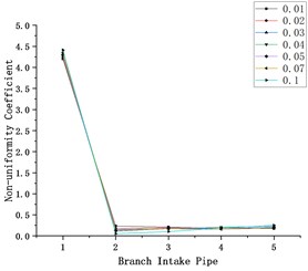
In engineering applications, the mass flow rate is usually controlled to control the amount of gas entering, and under the condition of gas density and pipeline area unchanged, the change of mass flow rate is shown as the change of gas velocity. In the premise of the model unchanged, select the flow of 0.01, 0.02, 0.03 and so on, a total of seven kinds of mass flow rate (unit: kg/s) for simulation. With the serial number of the branch intake pipeline as the abscissa and the flow nonuniformity coefficient as the ordinate (as shown in Fig. 4), the influence of gas velocity on the flow distribution uniformity was explored.

Fig. 4Influence of flow velocity on flow non-uniformity coefficient at each outlet

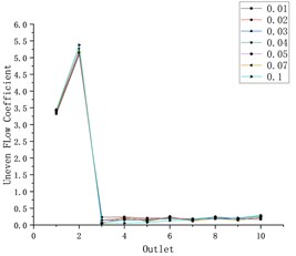
Combined with the flow diagram and velocity cloud diagram in CFD-POST, it can be found that when the gas enters from the air inlet, a large amount of gas flows out of the air inlet pipe 1, and the gas velocity flowing to the other four air inlet pipes decreases rapidly, and the gas velocity at the end of the pipe is close to zero. This phenomenon becomes more obvious with the increase of the mass flow rate of the gas.

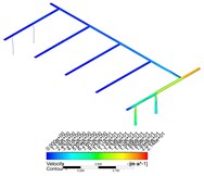
Fig. 5Velocity nephogram and streamline distribution under various flow conditions

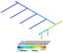
a) 0.01

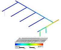
b) 0.02

c) 0.03

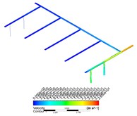
d) 0.04

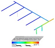
e) 0.05

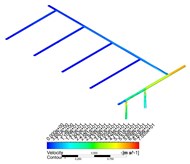
f) 0.1

With the increase of the mass flow rate of gas, under the condition of a certain inlet area, the entering speed of gas will be higher, and more gas will flow out of the pipeline connected with the inlet in a shorter time. When the high-speed airflow flows through a shunt tee, the sudden increase of local resistance will lead to the increase of frictional resistance and the decrease of gas velocity. According to the empirical formula, when the gas flow rate is higher, the resistance loss is greater, and the speed will decline faster, resulting in the decrease of the amount of gas flowing to the end of the pipe, and the uneven distribution of the flow of gas in other inlet pipes.

Add the outlet flow in each intake pipe, and Fig. 6 is obtained. It can be found from the analysis of Fig. 6 that the flow non-uniformity coefficient of gas in the first intake pipe is far more than 1, while the flow non-uniformity coefficient of other intake pipes fluctuates greatly due to the phenomenon of backflow.

Fig. 6Influence of flow velocity on flow non-uniformity coefficient at each branch inlet pipe

3.3. Influence of different inlet positions on flow distribution uniformity

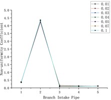
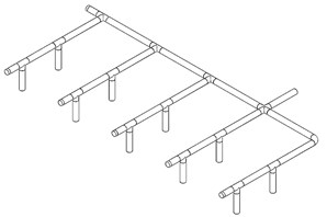
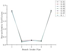
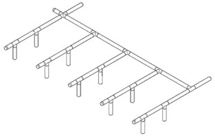
After adjusting the position of the air inlet, the simulation test was carried out again. The flow of each air outlet obtained was added according to the branch intake pipe, and Fig. 7 was obtained. Where Fig. 7(a) and 7(c) were the relation diagram of the flow non-uniformity coefficient and the branch intake pipe, Fig. 7(b) and 7(d) are the corresponding models of Fig. 7(a), 7(c).

By analyzing a and c, it can be found that no matter where the air inlet is in the pipeline, most of the gas entering from the air inlet will flow out of the branch air inlet connected with the air inlet. Compared with the model in which the air inlet is connected to the first air inlet, the model in which the air inlet is connected to the third air inlet has a better flow distribution uniformity, but it is far from the ideal state.

Fig. 7Influence of different inlet positions on flow distribution uniformity

a)

b)

c)

d)

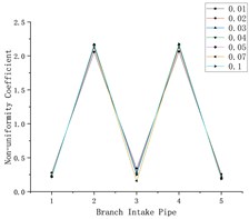
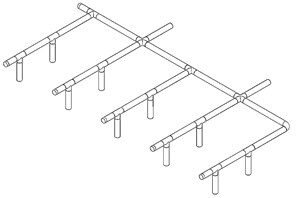
Fig. 8Influence of different number of air intakes on flow heterogeneity

a)

b)

c)

d)

3.4. Influence of different intake numbers on flow distribution uniformity

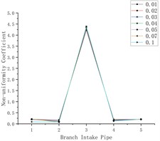
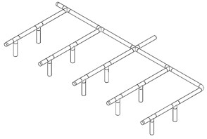
The number and position of air intakes were adjusted for simulation analysis again, and the flow of each air outlet was added according to the branch and air inlet pipes, and Fig. 8 was obtained. Where Fig. 8(a) and 8(c) were the relation diagram of the flow non-uniformity coefficient and the branch intake pipe, Figs. 8(b) and 8(d) are the corresponding models of Fig. 8(a) and 8(c).

Analyze Fig. 8(a) and 8(c), it can be found that although the number of air intakes is increased, the uneven flow distribution has not been greatly improved in essence. The uneven flow distribution coefficient of the branch intake pipeline connected with the air inlet is still much higher than that of other branch intake pipelines. Compared with the parallel pipe set model with only one air inlet, the parallel pipe set model with two air intakes can improve the uneven flow distribution phenomenon to a certain extent.