PSO optimum control strategy of 7 degrees of freedom semi-active suspensions

The performance of vehicle body vibration and ride comfort of active or semi-active suspension with proper control is better than that with passive suspension. It is important to use simple, reliable, effective and low-cost optimal control methods to control the vehicle suspension. An important issue in the optimal control of vehicle semi-active suspension is to determine the weighting coefficient reasonably. This paper established a whole-car model of semi-active suspension systems with 7 degrees of freedom in Matlab, built optimum control system with system function, and then optimized the weight of control system by Particle Swarm Optimization (PSO) [1]. The results show that under different road input, the seven-degree-of-freedom control model for the whole vehicle controlled by particle swarm optimization algorithm can obtain better control effect, and effectively improve the comprehensive performance of the semi-active suspension system, both the vehicle's ride comfort and handling stability.

1. Introduction

The suspension system is an important part of the vehicle, and its performance plays a decisive role in the ride comfort, operation, and stability. The passive vehicle suspension system was firstly presented by Olley in 1930s, which was generally composed of the stiffness-damping system. However, the parameters of passive vehicle suspension system could not be adjusted after they were determined. Normally, it cannot gain the satisfying performance in all of those three indexes or must rely on a complex structure [2], [3] Semi-active suspension can adjust suspension parameters according to the control strategy to achieve satisfying performance in different condition of the vehicle and the road [4]–[6]. And compared with active suspension, semi-active suspension has a simple structure and low cost advantages, which has been widely popularized in the market.

In practical vehicle suspension systems, the parameter uncertainties are usually unavoidable. To solve the problem, researchers have studied different modern control strategies. In addition to the traditional PID control strategy, they also adopt control strategies such as SDC (Skyhook Damper Control) [7], LQG (Linear Quadratic Gaussian) control [8], [9], fuzzy control [10], [11], SMC (Sliding Mode Control) [12], H∞ control [13], [14], adaptive control [15], [16], predictive control [17], [18], neural network control [19], [20], nonlinear intelligent control [21], and compound control [22], to reduce the vibration amplitude of vehicle body and improve the vehicle ride smoothness, stability, and ride comfort.

In the previous studies of active suspension control, PID control is often used as it has a simple principle and strong adaptability. However, it is not very effective in suspension systems with uncertain parameters. The above-mentioned traditional classic control methods have the characteristics of simple structure, reliable performance, and they are easy to implement in industry. However, under certain conditions, the system will have some problems such as delay and jitter, which will cause the system to be unstable. The system adopting the neural network control method needs to provide many labeled samples and consumes a lot of computing power. Moreover, these control algorithms are only applied to a quarter of the car model, and are not used in the simulation application of the 7-degree-of-freedom vehicle control model.

To solve the problem of the ride comfort and stability of the active suspension control system during the learning process, the passive suspension is still retained in the design of the suspension system. In order to make full use of the advantages of passive and active suspension force control and its practical application, a force control strategy for vehicle semi-active suspension system based on PSO optimization is proposed. The focuses of semi-active vehicle research are the development of adjustable damping shock absorbers, the study of control theory and methods, and the computer realization of operating systems. The control methods and controller design based on modern control theory are the cores of the semi-active suspension system research. The control strategy directly determines the performance of semi-active suspension. In the design of vehicle semi-active suspension, the optimal controller with different objective functions can be determined according to different performance requirements. Therefore, it’s important to determine the weighting coefficient reasonably for optimal control of vehicle semi-active suspension, because the selection of weighting coefficient in objective function decides the control effect of the control system itself.

The PSO algorithm is a new optimized computing technology derived from the study of bird predation behavior. It belongs to the category of stochastic global optimization technology, which is fast, effective and robust. In order to ensure the accuracy of the analysis results, this paper takes the automobile as the research object, establishes a seven-degree-of-freedom vehicle dynamics model in MATLAB, and designs the particle swarm optimization controller and different working conditions according to different working conditions. Under the vibration response of driving, the particle swarm algorithm is used to calculate the weight coefficient of each evaluation index in the optimal controller under different working conditions to meet the requirements of ride comfort and handling stability under different road grades.

2. Establishment of suspension system model

2.1. Pavement model establishment

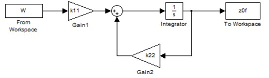
Based on the known power spectral density, the method of filtering white noise [23] is used to construct the time domain model of the road surface as follows:

1

{\dot{z}}_{g} (t) = - 2 π f_{0} z_{g} (t) + 2 π \sqrt{G_{q} (n_{0}) u} W (t) .

In the formula, $z_{g} (t)$ is pavement displacement, $f_{0}$ is lower cut-off frequency, $G_{q} (n_{0})$ is pavement roughness coefficient, $u$ is vehicle speed, $W (t)$ is filtered white noise. The generated model of filtered white noise random road spectrum established by Simulink tool kit is shown in Fig. 1.

Fig. 1Random filtering white noise random rode spectrum generation model

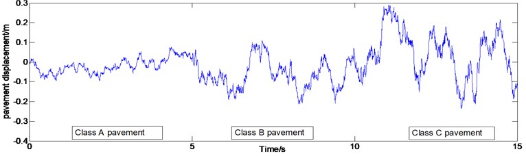
In Matlab, the white noise power $W_{h}$ is 20 dB [24], vehicle speed is 60 km/h, using three pavement grades of A, B and C, the road roughness coefficient $G_{q} (n_{0})$ is 1.6×10^-5m³/cycle, 6.4×10^-5 m³/cycle, 2.56×10^-4 m³/cycle, and the lower cut-off frequency is 0.068 Hz. The solver is fixed-step ode4 (Runge-Kutta) solver [25], and generated A, B and C grade road spectrum are shown in Fig. 2.

Fig. 2Integrated white noise method generated grade A, Band C road spectrum

2.2. Seven degrees of freedom vehicle model establishment

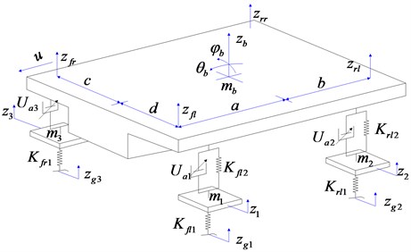
In order to simplify the dynamics modeling process, following the reasonable assumptions, a dynamic model of a semi-active vehicle suspension system with 7 degrees of freedom for a certain car is established as shown in Fig. 3 [26].

(1) With the exception of tires, suspension springs and shock absorber, the rest of the components are simplified to rigid bodies and no structural deformation occurs.

(2) The suspension system consists of a linear spring and a viscous damper. The wheel is simplified as a linear spring and it is always in contact with the ground.

(3) The body pitch angle is small, and the sprung mass center of mass is vertically moved relative to the road surface excitation.

(4) Ignore the coupling effects of the front and rear axles of the vehicle, that is, the suspension mass distribution coefficient is 1.

(5) Ignore the effects of non-linear factors such as tire vertical stiffness and suspension stiffness.

Through the analysis of the motion of the car, the dynamic equation of the system is as follows:

2

\{\begin{array}{l} m_{1} {\ddot{z}}_{1} = K_{f l 1} (q_{1} - z_{1}) + K_{f l 2} (z_{f l} - z_{1}) - U_{a 1}, \\ m_{2} {\ddot{z}}_{2} = K_{r l 1} (q_{2} - z_{2}) + K_{r l 2} (z_{r l} - z_{2}) - U_{a 2}, \\ m_{3} {\ddot{z}}_{3} = K_{f r 1} (q_{3} - z_{3}) + K_{f r 2} (z_{f r} - z_{3}) - U_{a 3}, \\ m_{4} {\ddot{z}}_{4} = K_{r r 1} (q_{4} - z_{4}) + K_{r r 2} (z_{r r} - z_{4}) - U_{a 4}, \\ m_{b} {\ddot{z}}_{b} = K_{f l 2} (z_{1} - z_{f l}) + K_{r l 2} (z_{2} - z_{r l}) + K_{f r 2} (z_{3} - z_{f r}) \\ + K_{r r 2} (z_{4} - z_{r r}) + U_{a 1} + U_{a 2} + U_{a 3} + U_{a 4}, \\ I_{p} {\ddot{θ}}_{b} = [K_{r l 2} (z_{2} - z_{r l}) + U_{a 2} + K_{r r 2} (z_{4} - z_{r r}) + U_{a 4}] \times b \\ - [K_{f l 2} (z_{1} - z_{f l}) + U_{a 1} + K_{f r 2} (z_{3} - z_{f r}) + U_{a 3}] \times a, \\ J_{r} {\ddot{φ}}_{b} = [K_{f l 2} (z_{1} - z_{f l}) + U_{a 1} + K_{r l 2} (z_{2} - z_{r l}) + U_{a 2}] \times d \\ - [K_{f r 2} (z_{3} - z_{f r}) + U_{a 3} + K_{r r 2} (z_{4} - z_{r r}) + U_{a 4}] \times c, \end{array}

where $U_{a 1}$ is the force of the left front wheel actuator, $U_{a 2}$ is the force of the left rear wheel actuator, $U_{a 3}$ is the force of the right front wheel actuator, $U_{a 4}$ is the force of the right rear wheel actuator.

Among them, $z_{f l} = - z_{b} + a θ_{b} + d φ,$ $z_{r l} = - z_{b} - b θ_{b} + d φ,$ $z_{f r} = - z_{b} + a θ_{b} - c φ,$ $z_{r r} = - z_{b} - b θ_{b} - c φ$ .

In the formula, $m_{1}$ is the left front wheel quality, $m_{2}$ is the left rear wheel mass, $m_{3}$ is the right front wheel quality, $m_{4}$ is the right rear wheel mass, $m_{b}$ is the body quality, $I_{p}$ is the body pitch moment of inertia, $J_{r}$ is the body roll moment of inertia, $K_{f l 1}$ is the left front wheel rigidity, $K_{r l 1}$ is the left rear wheel tire rigidity, $K_{f r 1}$ is the right front wheel stiffness, $K_{r r 1}$ the right rear wheel rigidity, $K_{f l 2}$ the left front wheel suspension stiffness, $K_{r l 2}$ is the left rear wheel suspension stiffness, $K_{f r 2}$ is the right front wheel suspension stiffness, $K_{r r 2}$ is the right rear wheel suspension stiffness, $C_{f l}$ is the left front wheel suspension damping, $C_{r l}$ is the left rear wheel suspension damping, $C_{f r}$ is the right front wheel suspension damping, $C_{r r}$ is the right rear wheel suspension damping, $a$ is the front axle to centroid distance, $b$ is the rear axle to centroid distance, $c$ is the right rear wheel center to centroid distance, $d$ is the left rear wheel center to centroid distance.

For the seven-degrees of freedom semi-active suspension dynamic model of the car, taking the system’s state variables $X = [{\dot{z}}_{1}, {\dot{z}}_{2}, {\dot{z}}_{3}, {\dot{z}}_{4}, {\dot{z}}_{b}, {\dot{θ}}_{b}, {\dot{φ}}_{b}, z_{1}, z_{2}, z_{3}, z_{4}, z_{b}, θ_{b}, φ_{b}]$ , control vectors $U_{c} = [U_{a 1}, U_{a 2}, U_{a 3}, U_{a 4}]$ , road disturbances $W = [z_{g 1}, z_{g 2}, z_{g 3}, z_{g 4}]$ , $U = [W; U_{c}]$ , output variables $Y = [{\dot{z}}_{1}, {\dot{z}}_{2}, {\dot{z}}_{3}, {\dot{z}}_{4}, {\dot{z}}_{b}, {\dot{θ}}_{b}, {\dot{φ}}_{b}, z_{1}, z_{2}, z_{3}, z_{4}, z_{b}, θ_{b}, φ_{b}]$ , and establishing the system’s state equation: $\{\begin{array}{l} \dot{X} = A_{l q r} X + B_{l q r} U, \\ Y = C_{l q r} X + D_{l q r} U . \end{array}$

Fig. 3Seven degrees of freedom vehicle model

3. Designing of optimal particle swarm optimization controller

3.1. Particle swarm optimization

The PSO algorithm can be understood as an iterative optimization tool. The system initializes a set of random solutions and iterative searches for the optimal value. In the PSO algorithm, each particle’s position $X_{j}$ represents a candidate solution to the optimization problem. The particles fly at a certain speed in the search space. This speed will dynamically adjust its flight direction and speed based on its own flight experience and the flight experience of its companions. All particles have a fitness value determined by the fitness function according to their current position (current position $X_{j}$ ) and the best position found so far (the individual extremum $P_{j}$ ). The particle searches in the solution space according to the current optimal particle, and finally finds the optimal position.

In the particle swarm optimization algorithm, it is firstly necessary to initialize the current position of the particle swarm and determine the objective function of the particle swarm optimization control. Then it needs to update the position, velocity, inertia weight and acceleration factor of the particle swarm according to certain rules, and update the iteration by recalculating the function of the target value particle and comparing the size of the particle [27]. Each variable in the particle is represented by a real number. The iterative steps of particle swarm optimization algorithm are as follows:

(1) There are $n$ particles in the $D$ -dimensional search space. During random initialization, the position and velocity of the $j$ -th particle are represented by $X_{i} = (X_{1, j}, X_{2, j} \dots, X_{d, j})$ and $V_{i} = (V_{1, j}, V_{2, j} \dots, V_{d, j})$ respectively;

(2) After evaluating the fitness of each particle and calculating the fitness value of the objective function, then store the current particle position and fitness value in each particle $P_{i} = (P_{1, j}, P_{2, j} \dots, P_{d, j})$ .

(3) Then calculate the individual extreme value. For each particle, compare the fitness value of the current position $X_{i}$ with the best position of the fitness of its own experience $P_{i}$ , if it is better than $P_{l}$ , its position will replace $P_{l}$ ;

(4) For the global extremum calculation, the fitness value of the local optimal position $P_{l}$ is compared with the fitness value of the best position $P_{g} = (P_{1, j}, P_{2, j}, \dots, P_{d, j})$ experienced in the group. If it is better than $P_{g}$ , the position will be replaced;

(5) Particle parameter update.

Update the inertia weight coefficient: $w (j_{s t e p}) = w_{m i n} + \frac{w_{m a x} - w_{m i n}}{i t e r} (i t e r - j_{s t e p})$ , where, $j_{s t e p}$ – current number of iterations, $w_{m a x}$ – maximum inertia factor, $i t e r$ – maximum evolutionary number, $w_{m i n}$ – minimum inertia factor.

Update accelerating factor: $c_{1} (j_{s t e p}) = (c_{1 e} - c_{1 j}) \frac{j_{s t e p}}{i t e r} + c_{1 j}$ , $c_{2} (j_{s t e p}) = (c_{2 e} - c_{2 j}) \frac{j_{s t e p}}{i t e r} + c_{2 j}$ , where, $c_{1 j}$ – the initial value of $c_{1}$ , $c_{2 j}$ – the initial value of $c_{2}$ , $c_{1 e}$ – the final value of $c_{1}$ , and $c_{2 e}$ – the final value of $c_{2}$ .

(6) Particle speed update.

Update the speed of particles:

V_{i, j} (j_{s t e p} + 1) = ω V_{i, j} (j_{s e p}) + c_{1} r_{1} [P_{i, l} - X_{i, j} (j_{s t e p})] + c_{2} r_{2} [P_{i, g} - V_{i, j} (j_{s t e p})],

(i = 1,2, \dots, d, j = 1,2, \dots, n) .

Determine if the new speed value is within the range: $V_{i, j} (j_{s t e p} + 1) \leq V_{m a x}$ , $i = 1,2, \dots, d$ , $j = 1,2, \dots, n$ .

If $v_{i, j}$ is greater than $v_{m a x}$ , use $v_{m a x}$ instead of $v_{i, j}$ ;

(7) Particle position update.

Substituting the updated velocity value into the formula:

X_{i, j} (j_{s t e p} + 1) = X_{i, j} (j_{s t e p}) + V_{i, j} (j_{s t e p} + 1), (i = 1,2, \dots, d, j = 1,2, \dots, n),

the new particle position value $x_{i, j}$ is obtained;

(8) Judge whether the termination condition is satisfied, and if it is satisfied, the process goes to step (8); otherwise, it goes to step (2) to continue the search calculation;

(9) Stop searching when the stop condition is met, output $P_{g}$ , end the seek operation.

3.2. Optimal controller design

The goal of the optimal control of semi-active suspension is to make the car get higher smoothness and control stability. If the vertical acceleration $Z$ value of the sprung center of mass is smaller, it means that the ride comfort of the vehicle is better. The evaluation index of vehicle handling stability mainly depends on sprung mass pitch angular acceleration, sprung mass lateral acceleration, suspension dynamic deflection, four-wheel dynamic load, etc. The smaller their value, the better the performance. Taking into account the complexity of the model and a large number of observations, the linear quadratic function of the semi-active suspension is defined as follows [28]:

3

\begin{array}{l} J = P_{1} {\ddot{x}}_{b}^{2} + P_{2} {\ddot{θ}}_{b}^{2} + P_{3} {\ddot{φ}}_{b}^{2} + P_{4} (z_{f l} - z_{1})^{2} + P_{5} (z_{r l} - z_{2})^{2} + P_{6} (z_{f r} - z_{2})^{2} \\ + P_{7} (z_{r r} - z_{4})^{2} + P_{8} (z_{1} - z_{g 1})^{2} + P_{9} (z_{2} - z_{g 2})^{2} + P_{10} (z_{3} - z_{g 3})^{2} + P_{11} (z_{4} - z_{g 4})^{2}, \end{array}

where $P_{1}$ , $P_{2}$ , $P_{3}$ , $P_{4}$ , $P_{5}$ , $P_{6}$ , $P_{7}$ , $P_{8}$ , $P_{9}$ , $P_{10}$ , $P_{11}$ are respectively the body acceleration, the pitch angle acceleration, the lateral inclination acceleration, the left front suspension dynamic stroke, the left rear wheel suspension dynamic stroke, the right front suspension dynamic stroke, the right rear wheel suspension dynamic stroke, the left front wheel tire change, left rear wheel tires deformation, right front tires deformation, the weighting coefficient of the deformation of the rear wheel tire, and written in the form of a matrix:

4

J = X^{T} Q X + U^{T} R U + 2 X^{T} N U,

where $Q$ and $R$ respectively represent the weighted matrices of the state variables and the control variables. The different values of $Q$ and $R$ allow the different weighting coefficients to be added to the different performance indexes in the function. For different performance requirements, a different optimal control feedback gain matrix can be obtained by changing the weighted coefficient matrix of the state variable and the control variable. And the controller can be designed to meet the requirements of different performance. In order to control the weighting coefficient matrix better, this paper proposes a particle swarm optimization algorithm to optimize the weighting coefficient of the optimal controller.

3.3. Designing of optimal controller for particle swarm

The semi-active suspension simulation model of Particle swarm optimal control is constructed as shown in Fig. 4.

Fig. 4The semi-active suspension simulation model of Particle swarm optimal control

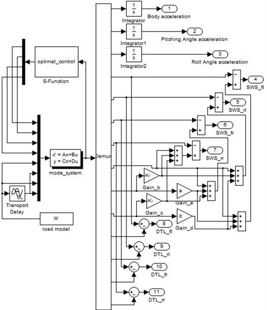
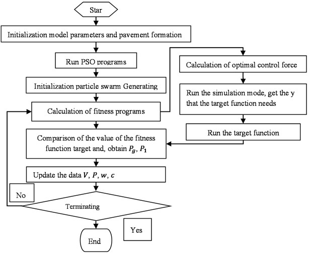
The operation block diagram of the optimal controller of particle swarm is shown in Fig. 5.

Fig. 5Simulation model of PSO-based best control strategy of semi-active suspensions

4. The optimal result subgroup of the optimal controller

According to the evaluation indexes corresponding to the vehicles on different roads, the fitness function corresponding to different road conditions is established, and the particle swarm algorithm is used to determine the weighting coefficient of each evaluation index. The relevant parameters of the vehicle model are shown in Table 1. These parameters, together with the parameters associated with the road, are programmed with Matlab and stored in the initial_parameters.m folder.

Table 1Model parameters of vehicle suspension system.

The parameter	The numerical	The parameter	The numerical
$m_{1}$ / kg	50	$C_{f l}$ / (kN / ms^-1)	1190
$m_{2}$ / kg	50	$C_{r l}$ / (kN / ms^-1)	1130
$m_{3}$ / kg	50	$C_{f r}$ / (kN / ms^-1)	1190
$m_{4}$ / kg	50	$C_{r r}$ / (kN / ms^-1)	1130
$m_{b}$ / kg	1300	$K_{f l 1}$ / ( kN.m^-1)	302342
$K_{f l 2}$ / (kN.m^-1)	19000	$K_{r l 1}$ / ( kN.m^-1)	492982
$K_{r l 2}$ / (kN.m^-1)	14700	$K_{f r 1}$ / ( kN.m^-1)	302342
$K_{f r 2}$ / (kN.m^-1)	19000	$K_{r r 1}$ / ( kN.m^-1)	492982
$K_{r r 2}$ / (kN.m^-1)	14700	$d$ / m	0.712
$I_{p}$ / (kg $\cdot$ m²)	2436	$c$ / m	0.712
$J_{r}$ / (kg $\cdot$ m²)	521	$a$ / m	1.219
$b$ / m	1.252

The test vehicle traverses A-C class roads at a speed of 60 km/h. Set the solver step size to ode4 (Runge-Kutta), and then run the program. The following Table 2 shows the optimized controller parameters.

Table 2Weighting coefficients under different levels of pavement

The weighted coefficient	The road level
The weighted coefficient	Class A pavement	Class B pavement	Class C pavement
$P_{1}$	2.13	4.56	4.23
$P_{2}$	0.36	1.03	0.16
$P_{3}$	8.55	4.59	5.61
$P_{4}$	23.2	36.6	11.7
$P_{5}$	18.7	28.4	12.8
$P_{6}$	21.3	35.2	19.8
$P_{7}$	29.6	24.5	12.8
$P_{8}$	2.12	1.88	0.91
$P_{9}$	2.88	1.95	0.51
$P_{10}$	2.68	1.78	0.26
$P_{11}$	2.15	1.78	0.34

5. Conclusions

In order to verify the accuracy of the vehicle model and the rationality and effectiveness of the control strategy, the semi-active suspension system was simulated and analyzed under different road conditions on the loop simulation platform. The test vehicle traverses A, B, and C roads at a constant speed of 60 km/h. The solver is seated to a fixed step length ode15 s (stiff/NDF) [29], and the simulation work step length is 0.02 s. The entire simulation time is 60 s, of which 0-20 s to A-class road, B-class road 20-40 s, and C-class road 40-60 s [30]. Through the particle swarm optimization algorithm of the semi-active suspension system, the body acceleration, pitch acceleration and roll acceleration are obtained. Their simulation results are shown in Figs. 6-7.

Fig. 6The characteristics of the body vertical acceleration in time domain

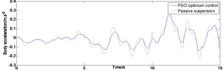
Fig. 7The characteristics of the pitch acceleration in time domain

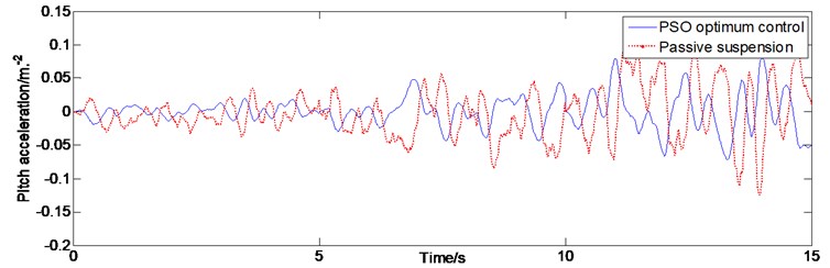
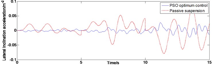
The evaluation index of car ride comfort is mainly the three axial weighted accelerations from the seat support points. More importantly, the human body is mostly affected by vertical vibration caused by uneven road surfaces. Therefore, in vehicle control, the vertical vibration at the center of mass of the vehicle body is extremely important. It can be seen in Fig. 6, compared with passive suspension, based on particle swarm optimal control of semi-active suspension system of vehicle body acceleration value in three grade pavement are much smaller than the passive suspension system. The pitch and roll movement of the vehicle also affect the comfort of the human body. It can be seen in Fig. 7 that the pitch acceleration has been controlled to a certain extent, and the control effect is still obvious. With the deterioration of traffic conditions, the pitch acceleration value of the C-level road is still controlled within a certain range. It can be seen from Fig. 8 that the lateral inclination acceleration has little effect on the change of the road slope, the acceleration values are all well attenuated, and the control effect is the most ideal. The simulation results show that the semi-active suspension controlled by the particle swarm optimization algorithm has a good control effect in the above three important degrees of freedom compared with the passive suspension. That means that the semi-active suspension controlled by the particle swarm optimization algorithm has a better attenuation effect, reducing the impact of the human body in the vertical vibration and roll and pitch movement of the vehicle body.

Fig. 8Characteristic diagram of lateral inclination acceleration in time domain

The simulation results of vehicle suspension system domain under random time road show that semi-active suspension based on particle swarm optimization control can effectively reduce the vertical vibration of vehicle acceleration on different levels of road surface. This shows that the particle swarm optimal controller can adjust the posture of the car body according to changes in traffic conditions. When the road conditions are poor, it can ensure driving safety while improving comfort and smoothness.

References

J. Kennedy and R. C. Eberhart, “Particle swarm optimization,” in Proceedings of IEEE International Conference on Neural Networks, pp. 760–766, 2011.

Search CrossRef
M. Z. Q. Chen, K. Wang, Y. Zou, and G. Chen, “Realization of three-port spring networks with inerter for effective mechanical control,” IEEE Transactions on Automatic Control, Vol. 60, No. 10, pp. 2722–2727, Oct. 2015, https://doi.org/10.1109/tac.2015.2394875

Publisher
K. Wang, M. Z. Q. Chen, and Y. Hu, “Synthesis of biquadratic impedances with at most four passive elements,” Journal of the Franklin Institute, Vol. 351, No. 3, pp. 1251–1267, 2014.

Publisher
X. Ma, P. K. Wong, J. Zhao, J.-H. Zhong, H. Ying, and X. Xu, “Design and testing of a nonlinear model predictive controller for ride height control of automotive semi-Active air suspension systems,” IEEE Access, Vol. 6, pp. 63777–63793, 2018, https://doi.org/10.1109/access.2018.2876496

Publisher
X. Tang, H. Du, S. Sun, D. Ning, Z. Xing, and W. Li, “Takagi-Sugeno fuzzy control for semi-active vehicle suspension with a magnetorheological damper and experimental validation,” IEEE/ASME Transactions on Mechatronics, Vol. 22, No. 1, pp. 291–300, Feb. 2017, https://doi.org/10.1109/tmech.2016.2619361

Publisher
M. Z. Q. Chen, Y. Hu, C. Li, and G. Chen, “Application of semi-Active inerter in semi-active suspensions via force tracking,” Journal of Vibration and Acoustics, Vol. 138, No. 4, pp. 1–11, Aug. 2016, https://doi.org/10.1115/1.4033357

Publisher
J. L. Yao, S. Taheri, and S. M. Tian, “A novel semi-active suspension design based on decoupling skyhook control,” Journal of Vibroengineering, Vol. 16, No. 3, pp. 1318–1325, 2014.

Search CrossRef
B. Lan and F. Yu, “Design and simulation analysis of LQG controller of active suspension,” Transactions of the Chinese Society of Agricultural Machinery, Vol. 35, No. 1, pp. 13–18, 2004.

Search CrossRef
Y. W. Yu, C. C. Zhou, and L. L. Zhao, “Design of LQG controller for vehicle active suspension system based on alternate iteration,” Journal of Shandong University, Vol. 47, No. 4, pp. 50–58, 2017.

Search CrossRef
R. W. Wang, X. P. Meng, and D. H. Shi, “Fuzzy control of vehicle ISD semi-active suspension,” Transactions of the Chinese Society of Agricultural Machinery, Vol. 44, No. 12, pp. 1–5, 2013.

Search CrossRef
D. Y. Wang and H. Wang, “Control method of vehicle semi active suspensions based on variable universe fuzzy control,” Chinese Journal of Mechanical Engineering, Vol. 28, No. 3, pp. 366–372, 2017.

Search CrossRef
J.-L. Yao, W.-K. Shi, J.-Q. Zheng, and H.-P. Zhou, “Development of a sliding mode controller for semi-active vehicle suspensions,” Journal of Vibration and Control, Vol. 19, No. 8, pp. 1152–1160, Jun. 2013, https://doi.org/10.1177/1077546312441045

Publisher
H. P. Du and N. Zhang, “Constrained H∞ control of active suspension for a half-car model with a. time delay in control,” Proceedings of the Institution of Mechanical Engineers, Part D: Journal of Automobile Engineering, Vol. 222, No. 5, pp. 665–684, 2008.

Publisher
W. Sun, H. Gao, and O. Kaynak, “Finite frequency H∞ control for vehicle active suspension systems,” IEEE Transactions on Control Systems Technology, Vol. 19, No. 2, pp. 416–422, Mar. 2011, https://doi.org/10.1109/tcst.2010.2042296

Publisher
W. Sun, Z. Zhao, and H. Gao, “Saturated adaptive robust control for active suspension systems,” IEEE Transactions on Industrial Electronics, Vol. 60, No. 9, pp. 3889–3896, Sep. 2013, https://doi.org/10.1109/tie.2012.2206340

Publisher
F. Zhao, S. S. Ge, F. Tu, Y. Qin, and M. Dong, “Adaptive neural network control for active suspension system with actuator saturation,” IET Control Theory and Applications, Vol. 10, No. 14, pp. 1696–1705, Sep. 2016, https://doi.org/10.1049/iet-cta.2015.1317

Publisher
M. Canale, M. Milanese, and C. Novara, “Semi-active suspension control using “fast” model-predictive techniques,” IEEE Transactions on Control Systems Technology, Vol. 14, No. 6, pp. 1034–1046, Nov. 2006, https://doi.org/10.1109/tcst.2006.880196

Publisher
D. Wang, D. Zhao, M. Gong, and B. Yang, “Research on robust model predictive control for electro-hydraulic servo active suspension systems,” IEEE Access, Vol. 6, pp. 3231–3240, 2018, https://doi.org/10.1109/access.2017.2787663

Publisher
S. H. Zhu, B. Z. Lv, and H. Wang, “Neural network control method of automotive semi-active air suspension,” Journal of Traffic and Transportation Engineering, Vol. 6, No. 4, pp. 66–70, 2006.

Search CrossRef
H. Li, Y. H. Feng, and L. Su, “Vehicle active suspension vibration control based on robust neural network,” Chinese Journal of Construction Machinery, Vol. 15, No. 4, pp. 324–337, 2017.

Search CrossRef
Y. Qin, J. J. Rath, C. Hu, C. Sentouh, and R. Wang, “Adaptive nonlinear active suspension control based on a robust road classifier with a modified super-twisting algorithm,” Nonlinear Dynamics, Vol. 97, No. 4, pp. 2425–2442, Sep. 2019, https://doi.org/10.1007/s11071-019-05138-8

Publisher
S. K. Sharma, U. Saini, and A. Kumar, “Semi-active control to reduce lateral vibration of passenger rail vehicle using disturbance rejection and continuous state damper controllers,” Journal of Vibration Engineering and Technologies, Vol. 7, No. 2, pp. 117–129, Apr. 2019, https://doi.org/10.1007/s42417-019-00088-2

Publisher
Fan Yu, “Vehicle Dynamics and Control,” Ph.D. Thesis, China Machine Press, Beijing, 2010.

Search CrossRef
Zhang Yufen, Long Jinlian, Li Jing, and Lu Jiaxuan, “Research on LQG of active suspension based on immune particle swarm optimization.,” Computer Engineering and Applications, Vol. 54, No. 6, pp. 252–256, 2018.

Search CrossRef
O. P. Agrawal and A. A. Shabana, “Application of deformable-body mean axis to flexible multibody system dynamics,” Computer Methods in Applied Mechanics and Engineering, Vol. 56, No. 2, pp. 217–245, Jun. 1986, https://doi.org/10.1016/0045-7825(86)90120-9

Publisher
Jun Yao and Songhui Ma, “Modeling and Simulation of Simulink,” Xidian University Press, Xian, 2009.

Search CrossRef
Andries Engelbrecht P., Fundamentals of Computational Swarm Intelligence. John Wiley and Sons, 2011.

Search CrossRef
X. Song and M. Ahmadian, “Characterization of semi-active control system dynamics with magneto-rheological suspensions,” Journal of Vibration and Control, Vol. 16, No. 10, pp. 1439–1463, Sep. 2010, https://doi.org/10.1177/1077546309103418

Publisher
Zhihong Guo, Konghui Guo, and Xiaolin Song, “Study of semi-active suspension control strategy based on an identification model,” Journal of Hunan University (Natural Sciences), Vol. 37, No. 12, 2010.

Search CrossRef
Xiaopeng Wang, Jianjun Liu, and Long Wu, “A simulation research on seven DOF semi-active full vehicle suspension,” (in Chinese), Journal of Hunan University of Technology, Vol. 30, No. 6, 2016.

Search CrossRef

Cited by

Influence of pneumatic tire enveloping behavior characteristics on the performance of a half car suspension system using multi-objective optimization algorithms

A.M. Kader | Hassan A. El-Gamal | Mohamed Abdelnaeem

(2024)

About this article

Received

31 July 2021

Accepted

20 November 2021

Published

15 December 2021

DOI

https://doi.org/10.21595/jmeacs.2021.22164

Keywords

semi-active suspension

particle swarm optimization

optimum control strategy

This is an open access article distributed under the Creative Commons Attribution License, which permits unrestricted use, distribution, and reproduction in any medium, provided the original work is properly cited.

Previous article in issue Previous Next article in issue Next

Research article

2023 08 22

Mechanism of time-delay feedback control of suspension damping with an annular vibration-absorbing structure

Yajie Chen, Kehui Ma, Chuanbo Ren, Yang Nan, Pengcheng Zhou

Research article

2019 08 15

Multi-objective optimization of active suspension predictive control based on improved PSO algorithm

Qiang Zhao, Baoquan Zhu

Research article

2018 12 31

Optimization design of semi-active controller for in-wheel motors suspension

Fangwu Ma, Jiawei Wang, Yang Wang, Longfan Yang

Research article

2017 06 30

Adaptive neural network control for semi-active vehicle suspensions

Zhushun Ding, Feng Zhao, Yechen Qin, Cheng Tan

J. Qiao, Y. Choi, and F. Yang, “PSO optimum control strategy of 7 degrees of freedom semi-active suspensions,” Journal of Mechanical Engineering, Automation and Control Systems, Vol. 2, No. 2, pp. 98–108, Dec. 2021, https://doi.org/10.21595/jmeacs.2021.22164

Copy Extrica

Copied to clipboard!

TY  - JOUR
DO  - 10.21595/jmeacs.2021.22164
UR  - https://doi.org/10.21595/jmeacs.2021.22164
TI  - PSO optimum control strategy of 7 degrees of freedom semi-active suspensions
T2  - Journal of Mechanical Engineering, Automation and Control Systems
AU  - Choi, Yeonsung
AU  - Qiao, Jubin
AU  - Yang, Fuqiang
PY  - 2021
DA  - 2021/12/15
PB  - JVE International Ltd.
SP  - 98-108
IS  - 2
VL  - 2
SN  - 2669-2600
SN  - 2669-1361
ER  - 

Copy Ris

Copied to clipboard!

@article{Choi_2021,
	doi = {10.21595/jmeacs.2021.22164},
	url = {https://doi.org/10.21595/jmeacs.2021.22164},
	year = 2021,
	month = {dec},
	publisher = {{JVE} International Ltd.},
	volume = {2},
	number = {2},
	pages = {98--108},
	author = {Yeonsung Choi and Jubin Qiao and Fuqiang Yang},
	title = {{PSO} optimum control strategy of 7 degrees of freedom semi-active suspensions},
	journal = {Journal of Mechanical Engineering, Automation and Control Systems}
}

Copy Bibtex

Copied to clipboard!

[1]Y. Choi, J. Qiao, and F. Yang, “PSO optimum control strategy of 7 degrees of freedom semi-active suspensions,” Journal of Mechanical Engineering, Automation and Control Systems, vol. 2, no. 2, pp. 98–108, Dec. 2021, doi: 10.21595/jmeacs.2021.22164.

Copy IEEE

Copied to clipboard!

Choi, Yeonsung, Jubin Qiao, and Fuqiang Yang. “PSO Optimum Control Strategy of 7 Degrees of Freedom Semi-Active Suspensions.” Journal of Mechanical Engineering, Automation and Control Systems 2, no. 2 (December 15, 2021): 98–108. https://doi.org/10.21595/jmeacs.2021.22164.

Copy Chicago

Copied to clipboard!

PSO optimum control strategy of 7 degrees of freedom semi-active suspensions

Abstract

1. Introduction

2. Establishment of suspension system model

2.1. Pavement model establishment

2.2. Seven degrees of freedom vehicle model establishment

3. Designing of optimal particle swarm optimization controller

3.1. Particle swarm optimization

3.2. Optimal controller design

3.3. Designing of optimal controller for particle swarm

4. The optimal result subgroup of the optimal controller

5. Conclusions

References

Cited by

About this article

Related Articles