Abstract
As one of the key components of the common rail system, the accuracy of pressure field and velocity field analysis of the common rail pipe is related to the service reliability. In order to obtain the velocity and pressure distribution that difficult to be measured in the experiment, this paper considers using three-dimensional modeling and establishing the three-dimensional model of oil flow in the common rail pipe based on the fluid simulation software, and then obtains the velocity field and pressure field distribution of the common rail pipe through numerical simulation. The cone angle at the nozzle structure of common rail pipe is compared and analyzed. Meanwhile the most appropriate cone angle’s processing angle among the commonly used processing cone angles is obtained, which improves the rationality of common rail pipe structure processing. It is great significance to the subsequent rail pressure stabilization analysis of common rail pipe.
Highlights
- Common rail pipe is one of the most important components for high-pressure fuel stability. The accurate analysis of its pressure field and velocity field is related to its working reliability. 3D modeling and simulation is a reliable method to effectively obtain its velocity and pressure distribution.
- In order to obtain the velocity and pressure distribution that difficult be measured in the experiment, the three-dimensional model of oil flow in the common rail pipe is established by using three-dimensional modeling and fluid simulation software. Then, the velocity field and pressure field of the common rail pipe are obtained by numerical simulation.
- The analysis of the influence of the common pipe structure on its pressure stabilizing performance focuses on the volume of the common rail pipe cavity, the length diameter ratio, the diameter of the damping hole, the length of the damping hole. In this paper, the influence of damping hole and nozzle structure formed at both ends on its pressure stabilizing performance is studied.
- The velocity and pressure distribution of common rail pipe under several commonly used machining cone angles are compared and analyzed, and the cone angle of nozzle structure with the best pressure stabilizing effect is obtained. The working reliability of this cone angle under different pressure conditions is further verified by changing the value of inlet pressure.
1. Introduction
Common rail pipe is the most important component for fuel pressure stability, which is the symbol that the high-pressure common rail system is different from the traditional fuel supply system. The common rail pipe separates the high-pressure pump from the injection system, so that the common rail system abandons the form of pressure control and time control and adopts the form of pressure time dual control, which is separated from the influence of engine operation on the injection process [1]. The volume of the common rail pipe, the diameter of the oil outlet and the structural form of the common rail pipe have a certain influence on the pressure stability in the common rail pipe. Therefore, the research on the fuel injection characteristics of common rail pipe will be of great significance to the optimal design of its structure and the key indexes such as economy, power, emissions and reliability of engine [2-4].
In this paper, ANSYS Workbench software is used to simulate and analyze the performance of common rail products for four cylinder gasoline engine manufactured by a fuel distributor manufacturing company. The damping hole at the high pressure oil inlet end and the nozzle structure formed at both ends are analyzed, which provides a basis for the optimization and improvement of structure.
2. Mathematical model and calculation method
In this paper, the flow problem of unsteady viscous fluid is considered. The fluid domain is in high pressure environment, and the flow field at the nozzle structure is in high turbulence state, so the turbulence model should be selected as the calculation model. Ignoring the problem of heat exchange on the fluid solid wall, in other word, ignoring the influence of temperature.
Fluid flow is governed by the law of conservation of physics. The basic conservation laws include the law of conservation of mass, the law of conservation of momentum and the law of conservation of energy. If the flow contains the mixing or interaction of different components, the system should also abide by the law of component conservation. If the flow is in a turbulent state, the system also follows an additional turbulent transport equation. The control equation is the mathematical description of these conservation laws [5, 6]. Any flow problem must meet the conservation law. Based on the above conservation law, combined with the sub model of turbulent motion, the physical boundary conditions and corresponding mathematical description are given on the meshed model, and the fluid motion state can be solved by numerical method [7].
In this analysis, the mass conservation equation and momentum conservation equation are used as the control equations, and the standard - model is selected as the calculation model.
Mass conservation equation:
where, is the oil density, is the quality source term.
Momentum conservation equation:
where, is static pressure, is the stress tensor, , is the gravity volume force and external volume force in the direction respectively.
- equation, equation:
where, represents turbulent kinetic energy, , represents the generation term of turbulent kinetic energy caused by average velocity gradient and buoyancy, respectively, is the Prandtl number corresponding to the turbulent kinetic energy, is the effect of pulsating expansion of compressible turbulence on the total dissipation rate, user defined source item.
equation:
where, represents the dissipation rate, , , is an empirical constant, is the Prandtl number corresponding to the dissipation rate, user defined source item, turbulent viscosity coefficient .
3. Numerical simulation
3.1. Common rail pipe model and meshing
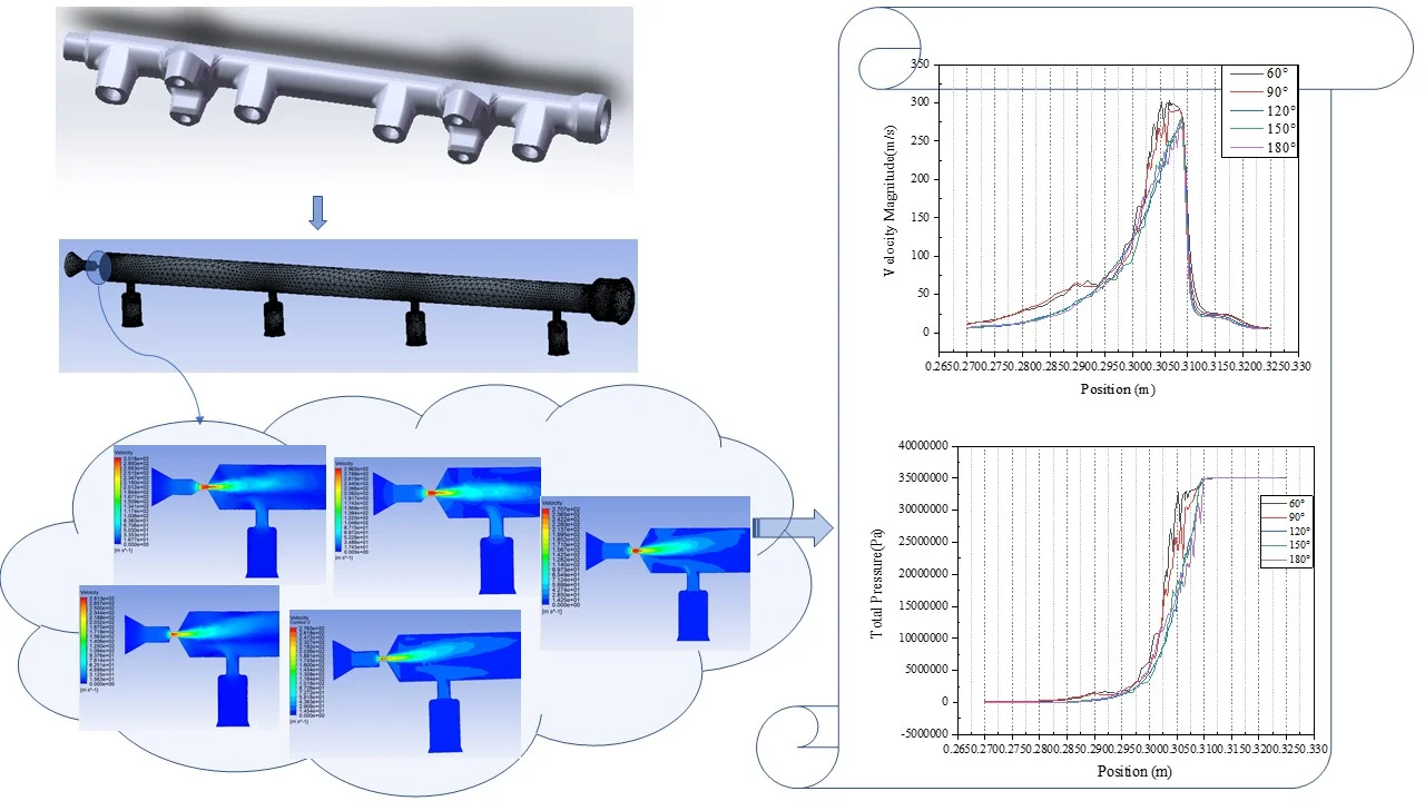
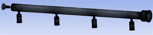
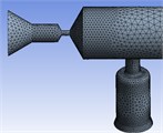
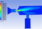
In terms of structure, the common rail pipe mainly includes the damping hole connecting the high-pressure oil pump end, the throttle hole connecting the fuel injector end, as well as the rail pressure sensor, pressure safety valve and flow limiting valve [8]. The physical model of the common rail pipe is shown in Fig. 1. Import the model into the workbench software, and use the channel extraction function of the software to extract the fuel fluid domain of the internal oil passage. When meshing, according to the structural characteristics of each part and the needs of calculation results, the element segmentation should be small and dense at the parts with large changes in section and curvature and the head deformation of common rail and common rail branches. For the parts with small changes in section and curvature as well as less important research objects (such as common rail pipe wall, common rail end, etc.), the element segmentation is relatively coarse. In this way, it can not only ensure the calculation accuracy requirements of key parts, but also reduce the calculation time [9].
Fig. 1Physical model of common rail pipe

The meshing function of the software is used to mesh the fluid body region, and the mesh is refined in small parts such as damping holes to improve the mesh accuracy. The division results are shown in Fig. 2(a), and Fig. 2(b) is the schematic diagram of local mesh refinement. The number of meshes in the fluid domain is 314457 and the number of nodes is 62115. The maximum deflection coefficient of the grid is 0.8253, the minimum is 0.2208 and the average is 0.1173. The maximum orthogonal coefficient of the grid is 0.997, the minimum is 0.1746 and the average is 0.7776. Based on the above parameters, it can be concluded that the mesh generation quality is good, and the next step of numerical simulation can be carried out.
Fig. 2a) Grid division model diagram of common rail pipe, b) grid refinement model diagram of local structure
a)
b)
3.2. Boundary condition setting
The simulation takes fuel as the medium, the fuel density is 730 kg/m3, and the viscosity is 0.0024 Pa·s. The inlet boundary condition adopts pressure inlet, the initial static pressure is 35 MPa, and the outlet boundary condition adopts pressure outlet.
4. Simulation result
4.1. Simulation results of pressure field and velocity field
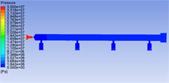
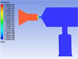
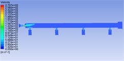
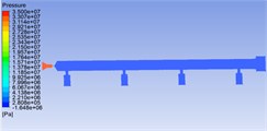
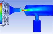
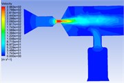
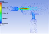
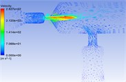
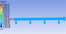
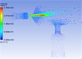
The central symmetry plane of the common rail tube is selected as the analysis object. It can be seen from the pressure cloud chart 3 and velocity cloud chart 4 that the pressure and velocity change dramatically in the nozzle throat. The pressure and velocity are evenly distributed in the cavity of the common rail tube.
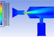
Fig. 4 shows that there is a phenomenon of partial oil backflow, and there is an obvious vortex formation at the tail of the nozzle structure. The vortex will change the direction of the flow rate of the fuel. In the vortex area, the fluid rotates, collides and backflows irregularly, which will cause great obstacles to the mainstream movement, consume the energy of the mainstream movement and produce flow pulsation, pressure loss. In the common rail tube cavity, the fluid has relatively enough space due to the relatively large volume. So that the fluid velocity and pressure can be fully developed, and then the distribution of fluid velocity and pressure in the common rail tube cavity is relatively uniform. In Fig. 3, there are unreasonable negative pressure values, which may be related to the grid division and initialization conditions, but because they are individual extreme values, they have little impact on the overall law analysis, so they can be ignored. Drastic changes mainly occur in the nozzle structure. If the structure here can be more reasonable, the pressure of the fluid entering the cavity can be quickly stabilized, which will improve the responsiveness of the whole common rail system, the working stability of the fuel injector and the smoothness of engine operation. There are three types of commonly used nozzles: cylindrical, conical, cone straight type [10]. The conical nozzle is difficult in the machining process, so I choose the cylindrical and cone straight type structure for comparative simulation analysis. The model used above is the cone straight type nozzle structure, and the cylindrical nozzle is equivalent to the cone straight type nozzle with a cone angle of 180°.
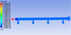
Fig. 3Pressure distribution cloud chart of common rail pipe
a)
b)
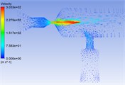
Fig. 4Velocity distribution cloud chart and velocity vector cloud chart of common rail pipe
a)
b)
c)
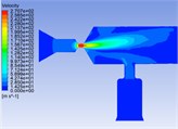
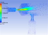
4.2. Simulation analysis of different cone angles
In this paper, the common rail tube of nozzle structure with cone angles of 60°, 90°, 150° and 180° is compared with the common rail tube with cone angle of 120° of the original nozzle structure. In order to eliminate the influence of volume, keep the volume at the nozzle structure unchanged, the length of damping hole unchanged, and the cone angle is the only variable. The simulation results are shown in the figure below.
Fig. 5Pressure distribution cloud chart, velocity distribution cloud chart and velocity vector cloud chart of common rail pipe with nozzle cone angle of 60°
a)
b)
c)
Fig. 6Pressure distribution cloud chart, velocity distribution cloud chart and velocity vector cloud chart of common rail pipe with nozzle cone angle of 90°
a)
b)
c)
Fig. 7Pressure distribution cloud chart, velocity distribution cloud chart and velocity vector cloud chart of common rail pipe with nozzle cone angle of 150°
a)
b)
c)
Fig. 8Pressure distribution cloud chart, velocity distribution cloud chart and velocity vector cloud chart of common rail pipe with nozzle cone angle of 180°
a)
b)
c)
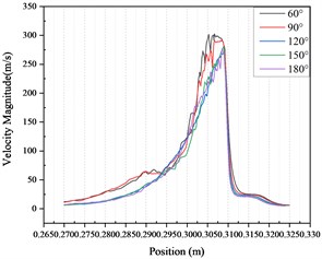
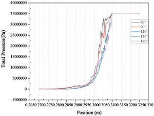
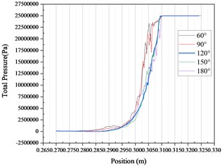
Fig. 9Velocity curve and pressure curve
a)
b)
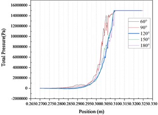
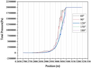
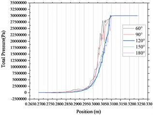
Fig. 10Pressure fluctuation curve under different pressure inlet conditions
a)
b)
c)
d)
Other conditions remain unchanged. Change the pressure value of the inlet pressure condition to obtain the pressure fluctuation curve in Fig. 10. It can be seen from the figure that under different pressure value inlet conditions, the common rail pressure curve with nozzle cone angle of 120° is still the most gentle and the fluctuation amplitude is the smallest.
It can be seen from the velocity cloud chart that the maximum value of velocity change occurs in the common rail pipe when the cone angle at the nozzle structure is 60°, and the minimum value of velocity change occurs in the common rail pipe when the cone angle at the nozzle structure is 120°. The velocity curve Fig. 9(a) and the pressure curve Fig. 9(b) are drawn from the simulation data. According to the velocity curve drawn from the simulation data, when the cone angle at the nozzle structure is 120°, the velocity change curve is the most gentle and the velocity fluctuation amplitude is the smallest. According to the pressure curve drawn from the simulation data, when the nozzle cone angle is 120°, the pressure curve changes the most gently and the pressure fluctuation amplitude is the smallest.
5. Conclusions
The flow of fuel in the common rail is a complex turbulent flow problem, which is a nonlinear fluid movement with irregular space and disordered time. Therefore, it is difficult to obtain the velocity and pressure distribution of fuel in the common rail pipe in the experiment. Using three-dimensional modeling combined with fluid software numerical simulation can fully simulate the fluid characteristics and obtain the velocity and pressure distribution that can better meet the actual conditions. By comparing some commonly used taper hole processing angles, it is analyzed that when the cone angle at the nozzle structure is 120°, the change of speed and pressure of the common rail pipe is gentler and the fluctuation range is small compared with other cone angles. Under the 120° cone angle, the pressure stabilization performance obstacle of the common rail pipe is small, the pressure will be stable faster, and the response performance is relatively best. Therefore, the 120° processing angle would be preferred when processing the cone angle.
References
-
Gu Huiya, Tang Yan, and Jiang Shunwen, “Analysis of structure for common-rail Based on AMESim,” Hydraulics Pneumatics and Seal, Vol. 4, pp. 16–18, 2010.
-
Kang Yanhong, Liu Xing, Wang Min, and Guo Haizhou, “Effect of the outlet oil hole on pressure fluctuation of the high-pressure common-rail system,” Internal Combustion Engines, Vol. 3, pp. 1–3, 2015.
-
Luo Zilai, Chang Hanbao, Zhang Xiaohuai, and Liu Boyun, “Simulation and experiment study of common rail pipe for marine heavy duty diesel engines,” Internal Combustion Engines, Vol. 6, pp. 37–39, 2012.
-
Dai Mengmeng and Zhang Yonghui, “Simulation investigation on effect ofpressure fluctuation in high pressure common rail on injection rate,” (in Chinese), Design and Manufacture of Diesel Engine, Vol. 19, No. 4, pp. 7–11, 2013.
-
J. N. Ding Xinshuo, Fluent Fluid Simulation Calculation. Beijing, China: Tsinghua University Press, 2013.
-
Han Zhanzhong, FLUENT – Example and Analysis of Fluid Engineering Simulation. Beijing, China: Beijing Institute of Technology Press, 2009.
-
Su Mingde, Fundamentals of Computational Fluid Dynamics. Beijing, China: Tsinghua University Press, 1997.
-
Wang Xinjun and Sun Dagang, “Simulation of CR system common – rail pipe,” Agricultural Equipment and Vehicle Engineering, Vol. 2, pp. 45–47, 2009.
-
Liu Feng, “Numerical simulation researches on the effects of the common rail parameters for the rail internal pressure field,” Small Internal Combustion Engine and Vehicle Technique, Vol. 43, No. 5, pp. 24–29, 2014.
-
Dong Zongzheng, Fu Biwei, Guo Can, and Xi Yan Qing, “Flow field simulation analysis of high pressure water jet nozzle based on CFD,” Petro and Chemical Equipment, Vol. 19, No. 7, pp. 20–23, 2016.
About this article

