Abstract
The integrated water distributor (IWD) is the adjustment terminal during the interval injection process. Its quality and performance are directly related to the effect of layered water injection. The IWD’s flow field is considered the research object, and the transient simulation is developed with Fluent dynamic grid and Fluid-Structure Interaction technology. The internal flow of the IWD during closing is simulated, and the mechanical behavior of the valve core is analyzed. The results show that: as the valve opening decreases, the high-speed areas appear at the throat of the valve core and the upper wall of the valve outlet; the throat of the valve presents a higher pressure gradient; the most serious deformation point appears on the lower side of the valve core, and the deformation increases as the valve core move down; the maximum equivalent strain occurs at the root of the valve core and increases as the valve core moves down.
1. Introduction
The integrated water distributor (IWD) is the adjustment terminal during the interval injection process. Its quality and performance are directly related to the effect of layered water injection [1].
Because of the influence of the IWD valve on the flow field, researchers have conducted a large number of experiments and simulation studies [2-5]. Guo [6] based on the theory of multi-rigid body kinematics and modal analysis, and used virtual prototype technology to study the dynamic characteristics of the actuator of the electronically controlled water distributor. Wang [7] established the corresponding mechanical model and imported the Simulink hydraulic simulation results of the pressure of the left piston cavity into ADAMS for dynamic simulation, and carried out research on the adjustment characteristics of the water distributor, such as the pressure difference between the start and the adjustment, the stroke of the control valve and the stable adjustment time. Meng [8] designed the test experiment process, conducted flow test experiments under different displacements for the cableless intelligent water distributor, and established a pipeline flow simulation model of the cableless intelligent water distributor.
At present, IWD is widely used in practical engineering, but the research on the transient flow characteristics of IWD is not enough. In this paper, the instantaneous flow during value closing is simulated, and the mechanical behavior of the valve core is analyzed. The research conclusions will provide a reference for evaluating the operational safety of water distributors.
2. Numerical model
2.1. Mathematical model
To order to analyze the flow inside IWD, the mass conservation equation and momentum conservation equation should be solved first. In addition, the equation of flow should be considered to calculate the outlet flux. The equation of flow rate through IWD is shown as:
where represents the cross-sectional area of fluid passageway in the valve (m2); represents the pressure difference about before the valve and after the valve (MPa); represents the density of fluid (kg/m3); represents the flow rate(m/s); represents the total local resistance factor.
The continuity equation is shown as:
where , , represents the speed in the , , directions, respectively (m/s).
The motion equation is used to describe the properties of fluid flow momentum conservation. For a Newtonian fluid, the Navier-Stokes equation can be obtained by introducing the constitutive equation of the fluid, which is shown as follows:
where represents velocity of fluid (m/s); represents dynamic viscosity coefficient of fluid ( s/m2); represents force of gravity in direction (m/s2).
2.2. Geometric model
Fig. 1 shows the 3D geometric model of the IWD, the material of the valve core is structural steel. The fluid enters the low field of the IWD from the inlet. The inlet pressure is 18.5MPa, while the outlet pressure is 17.1 MPa. In the numerical simulation, the flow field and the valve core need to be calculated simultaneously. Therefore, the flow field in the geometric model needs to be extracted for CFD simulation and analysis.
Because of the complexity of IWD, automatic mesh generation is adopted. The original structure is selected as the model to carry out the independent verification, which is shown in Table 1. From Table 1, the model whose grid number is 58973 is selected as the most appropriate meshing way.
Fig. 1Geometric model of the integrated water distributor [1]
![Geometric model of the integrated water distributor [1]](https://static-01.extrica.com/articles/22548/22548-img1.jpg)
Table 1Grid independent verification
(104) | 1.8972 | 2.5975 | 3.7761 | 5.8973 | 7.6123 |
Flux (Max) | 284.99 | 279.41 | 280.63 | 281.55 | 282.12 |
Flux (Min) | 279.47 | 273.09 | 276.66 | 273.71 | 272.56 |
Flux (Ave) | 282.23 | 276.25 | 278.64 | 277.63 | 277.34 |
2.3. Moving mesh algorithm and UDF coding
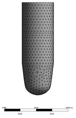
According to the closing feature of the valve core, the moving mesh algorithm is used to process the movement process of the valve core[9]. The grids of the fluid computational domain and the solid computational domain after grid independence verification are shown in Fig. 2 and Fig. 3, respectively.
Here DEFINE_CG_MOTION is used to define the movement of the valve core, the movement speed of the valve core is set to be 0.008 m/s.
Fig. 2Grid of fluid computational domain
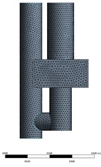
Fig. 3Grid of solid computational domain
2.4. Boundary conditions
The working fluid is water. The unsteady numerical simulation method is adopted. The flow governing equation is closed with the help of the standard - turbulence model, and the SIMPLE algorithm is used to solve the flow governing equation. The method uses a second-order upwind style to discretize the equations in parallel grid nodes to ensure the accuracy of the simulation results. The pressure inlet and pressure outlet boundary conditions are used for the computational domain, the initial valve pressure is set to 18.5 MPa, the outlet pressure is set to 17.1 MPa, and the turbulence intensity is set to 5 %.
2.5. Fluid-structure interaction settings
This paper uses the two-way FSI technology of the commercial software ANSYS Workbench to solve the problem. The Fluent and Mechanical respectively perform implicit iterative solutions to the flow field and structural field in each time step, while data (displacement, velocity, and acceleration) have interacted through preset fluid-structure interaction interfaces.
3. Simulations and results
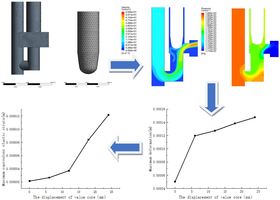
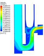
Fig. 4 shows the velocity distribution at different times during the closing process of the valve core. It can be seen from Fig. 4(a) that in the initial stage of valve closing, the valve core has little effect on the flow field characteristics. The high-speed fluid is injected into the inlet, hits the U-shaped pipe wall, rebounds, and then moves toward the outlet. As the outlet section becomes smaller, high-speed areas are gradually formed in the throat and the outlet, and an obvious low-speed area is formed on the underside of the valve core, which is related to the deflection of the flow and the shape of the wall.
As the valve opening decreases, the flow velocity at the throat becomes higher, the maximum velocity reaches about 58.5 m/s, and an apparent velocity gradient is formed. Due to the structural characteristics of the valve core, the fluid flows along the valve core wall after rushing out of the throat, then rebounds after hitting the upper wall and converges to form a second high-speed area. When the valve opening continues to decrease (as shown in Fig. 4(d)), the energy decay of the fluid reduces the flow rate in the two high-speed regions to 43 m/s and 45 m/s, respectively. When the valve is closed, the overall speed is reduced, and the two high-speed zones still exist, but the maximum speed is 12m/s and 14m/s, respectively. speed is 12 m/s and 14 m/s, respectively.
Fig. 4Instantaneous velocity distributions during valve-closing process
a)

b)

c)

d)

e)
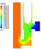
Fig. 5Instantaneous pressure distributions during valve-closing process
a)

b)

c)

d)

e)
Fig. 5 shows the pressure distribution during valve closing. At the initial stage (Fig. 5(a)), a high-pressure area is formed at the U-shaped pipe, and pressure gradients are formed at the U-shaped pipe and outlet, respectively (Fig. 5(b)). As the valve opening decreases (Fig. 5(c)), the valve core's effect on the flow increases, and the low-pressure region extend to the lower right corner of the valve core. A high-pressure area is formed at the upper wall, which is caused by the sudden change of the flow direction [10]. As the opening continues to decrease (Fig. 5(d)), the pressure distribution in the U-shaped pipe tends to be uniform, and the movement of the valve core makes the outlet flow section smaller, but still maintains a high-pressure difference at the throat. As the fluid energy is weakened, the high-pressure area on the upper wall of the outlet is reduced. The pressure distribution in the outlet pipe corresponds to the velocity distribution. During the valve closing process, the pressure in the inlet U-shaped pipe increased significantly, and the pressure gradient drop area gradually shifted to the throat.
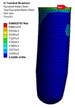
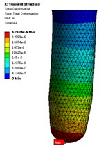
Fig. 6The deformation and the equivalent elastic strain distribution of the valve core (t= 1.5 s)
a)
b)
Fig. 7 shows the maximum equivalent strain of the valve core with different displacements during valve closing. During the downward movement of the valve core, the maximum equivalent stress on the valve core gradually increases. When the valve core displacement is 25 mm, the maximum equivalent stress is the largest, about 1.2159e-2 mm. As the valve continues to move down, the pressure in the U-tube rises and the maximum equivalent stress increases. Due to the downward movement of the valve core, the pressure in the U-shaped pipe is very high, so the maximum equivalent stress is large. Fig. 6(a) shows the maximum equivalent strain distribution of the valve core when the displacement is 12 mm. It can be seen from the figure that the maximum equivalent stress on the valve core appears in the root region of the valve core, and the maximum equivalent strain is about 3.7124e-1 mm.
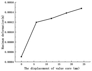
Fig. 8 shows the maximum deformation of the valve core during the valve closing process. It can be seen that the maximum deformation increases with the downward movement of the valve core. In the initial stage, the deformation of the valve core is small, as the valve core moves down, the displacement of the valve core increases under the action of the fluid on the valve core. Fig. 6(b) shows the deformation distribution of the valve core when 1.5 s. It can be seen from the figure that the maximum deformation occurs at the position on the right side of the valve core close to the inner wall of the valve cavity, and the maximum deformation is about 0. 015 mm. As the valve continues to move down, when the fluid passes through the outlet pipe, the valve core is squeezed, and the right side of the valve core is squeezed, resulting in large deformation. The amount of deformation decreases from the lower right side of the valve core to the upper left side, and the layered distribution of the deformation amount is obvious.
Fig. 7Maximum equivalent elastic strain of different valve core displacements
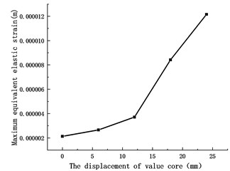
Fig. 8Maximum deformation of different valve core displacements
4. Conclusions
1) In the initial stage of valve closing, a local high-speed area and a pressure gradient area appear at the outlet. When the opening decreases, the high-speed area separates, the flow velocity at the throat increases significantly, and the pressure gradient here is formed. The impact of the fluid makes the upper wall of the outlet form a high-velocity area and low-pressure area.
2) During the valve closing process, the maximum deformation of the valve body occurs at the lower right end of the valve core. As the valve core moves down, the maximum deformation value increases. The maximum equivalent strain appears at the upper end of the valve core and increases with the decrease of the opening.
References
-
H. Liu, X. Pei, D. Jia, F. Sun, and T. Guo, “Connotation, application and prospect of the fourth-generation separated layer water injection technology,” Petroleum Exploration and Development, Vol. 44, No. 4, pp. 644–651, Aug. 2017, https://doi.org/10.1016/s1876-3804(17)30073-3
-
D. Jia, X. Pei, H. Liu, C. Cui, Y. Yu, and M. Liu, “A novel DC power line carrier technology for the technological process of water distributor in water injection well,” International Journal of Smart Home, Vol. 8, No. 6, pp. 37–44, Nov. 2014, https://doi.org/10.14257/ijsh.2014.8.6.04
-
H. Liu, X. Pei, K. Luo, F. Sun, L. Zheng, and Q. Yang, “Current status and trend of separated layer water flooding in China,” Petroleum Exploration and Development, Vol. 40, No. 6, pp. 785–790, Dec. 2013, https://doi.org/10.1016/s1876-3804(13)60105-6
-
X. H. Kong, D. T. Lu, and C. Y. Lin, “Numerical simulation of flow fields for water injectors.,” (in Chinese), Journal of Hydrodynamics, Vol. 22, No. 1, pp. 1–8, Jan. 2014, https://doi.org/10.3969/j.issn.1000-4874.2007.01.001
-
X. Zhou and Y. U. Minchao, “Dynamic characteristics analysis of eccentric quantitative water allocation based on Simulink.,” (in Chinese), Machine Tool and Hydraulics, Vol. 40, No. 11, pp. 54–56, Jun. 2012, https://doi.org/10.3969/j.issn.1001-3881.2012.11.016
-
S. J. Guo, J. Fan, and X. D. Fu, “Study on dynamic characteristics of electronically-controlled-type water distributor,” (in Chinese), Machinery Design and Manufacture, Vol. 87, No. 10, pp. 240–242, Oct. 2012, https://doi.org/10.19356/j.cnki.1001-3997.2012.10.087
-
N. Wang et al., “Simulation analysis on real-time adjusting distributor based on ADAMS,” (in Chinese), China Petroleum Machinery, Vol. 44, No. 7, pp. 113–116, Apr. 2016, https://doi.org/10.16082/j.cnki.issn.1001-4578.2016.07.024
-
S. K. Yang, G. Y. Zhao, X. F. Li, H. F. Guo, X. X. Du, and Z. H. Liao, “Optimization and evaluation of water nozzle structure of intelligent stepless regulating water distributor in water injection well,” (in Chinese), HENAN SCIENCE, Vol. 29, No. 2, pp. 113–116, Feb. 2021, https://doi.org/10.3969/j.issn.1004-3918.2021.02.004
-
Z. Lin, C. Ma, H. Xu, X. Li, B. Cui, and Z. Zhu, “Numerical and experimental studies on hydrodynamic characteristics of sleeve regulating valves,” Flow Measurement and Instrumentation, Vol. 53, pp. 279–285, Mar. 2017, https://doi.org/10.1016/j.flowmeasinst.2016.12.001
-
B. Kai and Q. Liu, “The numerical analysis and optimization design for throttle valves based on fluid-soild coupling workbench,” (in Chinese), Machine Design and Research, Vol. 30, No. 4, pp. 116–119, 2017, https://doi.org/10.13952/j.cnki.jofmdr.2014.0111
About this article

This work is supported by the Research on the Fluid Flow and the Design Method of Multi-functional Subsea Pipeline Robot (Grant No. U1908228).
