Abstract
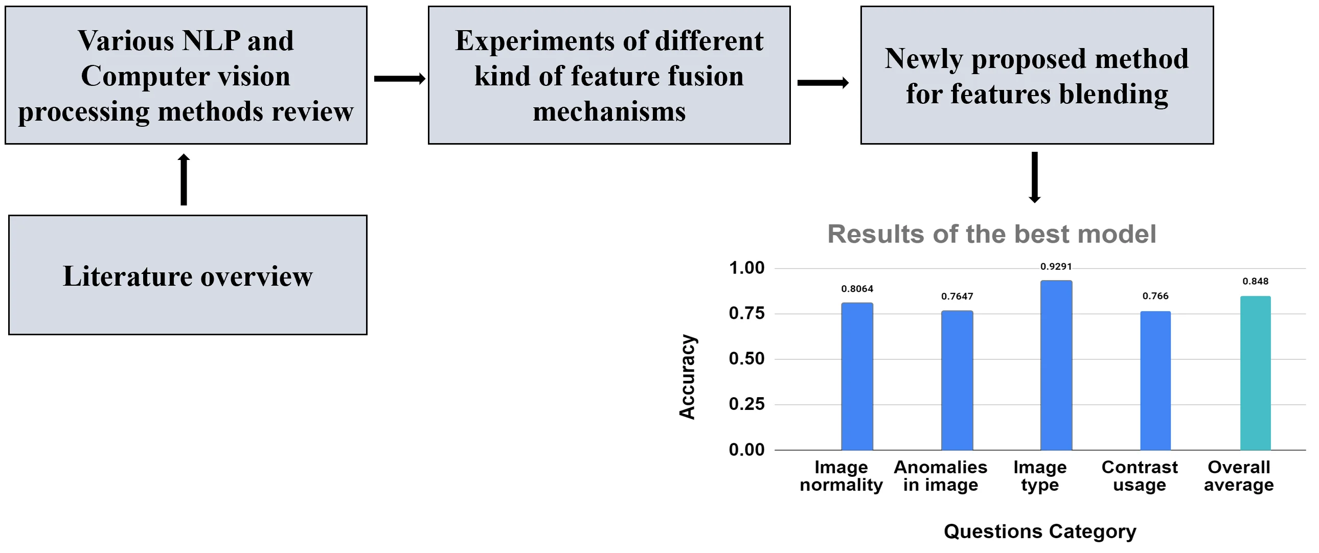
Computer vision applications in the medical field are widespread, and language processing models have gained more and more interest as well. However, these two different tasks often go separately: disease or pathology detection is often based purely on image models, while for example patient notes are treated only from the natural language processing perspective. However, there is an important task between: given a medical image, describe what is inside it – organs, modality, pathology, location, and stage of the pathology, etc. This type of area falls into the so-called VQA area – Visual Question Answering. In this work, we concentrate on blending deep features extracted from image and language models into a single representation. A new method of feature fusion is proposed and shown to be superior in terms of accuracy compared to summation and concatenation methods. For the radiology image dataset VQA-2019 Med [1], the new method achieves 84.8 % compared to 82.2 % for other considered feature fusion methods. In addition to increased accuracy, the proposed model does not become more difficult to train as the number of unknown parameters does not increase, as compared with the simple addition operation for fusing features.
Highlights
- One of the major unsolved issues in the Visual Question Answering field is finding the best way of fusing features from image and text models
- In this paper, a method of feature fusion is proposed, which allows extraction of a larger amount of possible interactions yet without increasing the number of unknown model parameters
- A new method of feature fusion was shown to be superior in terms of accuracy compared to summation and concatenation methods
1. Introduction
According to World Health Organization data in 2021 more than 45 % of world countries had less than one physician for 1,000 residents [2]. For this reason, medical personnel is forced to work a large number of hours, and this situation leads to a growing human error rate. Since the physician’s work requires a lot of time to analyze medical images, deep learning could come to hand and automate image processing. Nowadays, machine learning researchers invest more and more attention into visual question answering problems and these endeavors lead to models which can understand the wider context of a given image and solve problems that require human-level reasoning. However, one of the major unsolved issues in the VQA field is the finding the best way of fusing features from two types of models: the language model (mostly based on recurrent networks) and the image model (often different flavors of CNN-type architectures). It is not a priori known which language features interact with which image features. One possibility is to take into account all possible interactions through the Hadamard product [3]. However, this approach is impractical, as the number of unknown parameters increases rapidly with the size of the language/image features. The simplest approach is to sum language and image feature vectors, but the information about possible interactions between different features is almost completely lost. Concatenation or multiplication fusion operations allow to retain slightly more information about interactions, but not enough to significantly improve the behavior of the model.
In this work, the authors propose a method of feature fusion, which allows extraction of a larger amount of possible interactions yet without increasing the number of unknown model parameters, e.g. for EfficientNetB0 and LSTM backbones when the simplest fusion strategy of adding features is used, the number of model parameters is 12 899 762, while using the proposed more complex way of feature blending even slightly decrease the number of unknown parameters to 12 108 710. In what follows, it is demonstrated how this strategy improves model accuracy on the VQA-2019 Med dataset.
2. Literature review
In [4] researchers in radiology VQA domain used VGG-16 convolutional neural network and global average pooling strategy for visual information feature vectors calculations, while for natural language processing BERT model was chosen. For fusing textual and visual information, authors implemented a Co-attention mechanism whose goal is to highlight the most important information while suppressing less relevant signals followed by multimodal factorized bilinear pooling. This architecture was trained on high-diversity radiology images and was able to reach a BLEU score equal to 0.644 by effectively avoiding the overfitting issue. For the same domain [5] used a stacked attention network and compact multimodal bilinear pooling. For both architectures, experiments were made using convolutional neural networks for image processing: the stacked attention network used VGG-16, while the multimodal compact bilinear pooling idea was based on ResNet-152 and ResNet-50 with ImageNet weights. For natural language processing, authors applied long-short-term memory networks without pre-trained embeddings. Note that the stacked attention network effectively took advantage of correlations between question and image regions tokens followed by multi-modal pooling for question and image combination extraction. Other authors [5] have shown that for radiology image-question pairs stacked attention network give better WBBS and BLEU metrics (0.174 and 0.121 corresponding). [6] proposes variational autoencoder models for visual question-answering in the radiology domain that take questions and digital images as input and generate answers. The main structure of this model consists of an encoder and decoder: the first one (convolutional neural network with long-short-term memory network) is responsible for creating latent space variables from image and question information, while the encoder, which is constructed from a multilayer perceptron, reconstructs latent space variables and then passes them to the LSTM decoder to generate an answer. In addition, [6] introduces a model for the VQA task based on image classification by removing natural language processing (since data have repetitive tendencies) and simplifies the entire task into a multiclass image classification problem, which is solved by the ResNet-50 backbone with the last custom Softmax layer. In [7] Inception-Resnet-v2 is combined with Bi-LSTM for the VQA task in the medical domain. The authors use mentioned architectures for image and textual feature vectors calculation, then combine them with concatenation operation and send resulting vector to the Bi-LSTM layer, whose output becomes the input for the fully connected layer with softmax activation for final prediction.
From the method review, it can be seen that many researchers use convolutional neural networks and recurrent neural networks for image and text feature vectors combination, then different mechanisms combine these vectors and send them to the final classification phase. From the diversity of fusion mechanisms, can be seen growing community interest in VQA problems which leads to more accurate and higher-level reasoning models.
3. Methods used
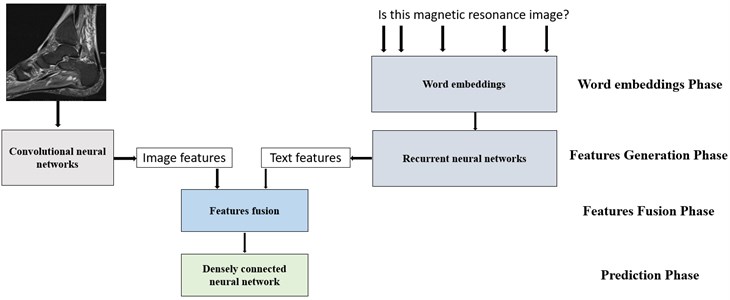
In Fig. 1 we provide a general scheme of the algorithm used in this work. For solving the VQA problem, the following architectures were selected: ResNet50V2, EfficientNetB0 for visual feature calculation, recurrent neural networks, and long-short-term memory neural networks for natural speech feature generation. In the following sub-chapters, we will introduce the main ideas and aspects of these models.
Fig. 1Scheme of visual question answering algorithm
3.1. Natural language processing methods
In this research, the experiments were based on the Skip-n-gram model, recurrent, long-short-term memory neural networks. These models will be introduced in the following sections.
3.1.1. Skip n-gram model
The goal of this model is to embed words into latent space in such a way that similar semantic meaning words would be as close as possible in a metric space, contrary to words with different semantic meanings. [8] provided a model based on the idea that similar semantic meaning words stay close to each other and maximize the probability that a given target word will be successfully identified by words around the input word (Fig. 2).
Fig. 2Scheme of the Skip n Gram model [8]
![Scheme of the Skip n Gram model [8]](https://static-01.extrica.com/articles/22737/22737-img2.jpg)
The algorithm of that model can be split into the following steps:
1) all words embedded in one-hot encoding vectors;
2) the one-hot encodings become input for the projection layer that maps the word to its embedding vector ;
3) the word vector is multiplied by the weights matrix and after applying the softmax context words, the, the probability distribution is obtained.
The model seeks to maximize the likelihood function:
here – context words, – target words, – weights matrix.
In addition, the probability that a context word remains near the target word can be calculated as follows [9]:
where, – count of unique words, means the th word position in the output vector, and is for the position of the word context in the output vector.
It is easy to accommodate minibatch situations often found in stochastic gradient-based optimization schemes when used for large datasets. All the notation remains the same, while is used to describe the batch size, and describes the count of context words. Thus, the batch log-likelihood function is as follows:
3.1.2. Recurrent neural networks
One of the biggest drawbacks of densely connected neural networks is that these models do not perform well on sequential data. In other words, the network cannot remember information about the previous input. When we are analysing natural language data, we can clearly understand that to generate features with textual semantic meaning, the network must understand sentences as sequential data and not as independent words. Thus, we are using recurrent neural networks instead of densely connected networks (Fig. 3). RNNs will be used to learn and extract deep features from the textual information that comes together with medical images.
Fig. 3a) Folded recurrent neural network; b) unfolded recurrent neural network (many to one) [10]
![a) Folded recurrent neural network; b) unfolded recurrent neural network (many to one) [10]](https://static-01.extrica.com/articles/22737/22737-img3.jpg)
a)
![a) Folded recurrent neural network; b) unfolded recurrent neural network (many to one) [10]](https://static-01.extrica.com/articles/22737/22737-img4.jpg)
b)
Recurrent neural networks of many to one type can be expressed by Eq. (4)-(5) [10]:
here , are activation functions, bias terms, W hidden layer weights matrix, U input weights matrix, V output vector weights matrix, hidden layer vector, output vector.
3.1.3. Long-short-term memory networks
Since recurrent neural networks often face vanishing or exploding gradient problems, long-short-term memory networks introduce forget, input, and output gates, which can drop irrelevant information and highlight the most relevant semantic information in a provided sentence [10].
Fig. 4LSTM network with 2 layers [11]
![LSTM network with 2 layers [11]](https://static-01.extrica.com/articles/22737/22737-img5.jpg)
Fig. 5Structure of the LSTM cell [12]
![Structure of the LSTM cell [12]](https://static-01.extrica.com/articles/22737/22737-img6.jpg)
The long-short-term memory network (Fig. 4, Fig. 5) can be expressed as the following equations [11]:
where denotes Hadamard operation, standard matrix multiplication, – forget gates, – input gates, – output gates, – cell activation vector, – cell vector, – hidden vector. – sigmoid activation function, – hyperbolic tangent activation function. , , , , , , , weight matrixes, o , , , bias terms. input vector.
3.2. Visual information processing methods
For visual feature calculation, ResNet and EfficientNet architectures were selected. Below, a brief introduction to these types of architecture is provided.
3.2.1. ResNet convolutional neural network architecture
Similarly, as recurrent neural networks, convolutional neural networks often face the problem of vanishing gradients. First, this drawback was partially solved by adding batch-normalization layers, which allowed one to partially alleviate the vanishing gradient problem. However, by adding more and more layers to the network, researchers faced again a gradient degradation problem. In 2015 [13] the authors proposed a new architecture idea which introduced residual connections. The main advantage of this modification is that this allows the network to learn residual mappings and if the gradients do vanish at some intermediate layer, the flow of gradients is not stopped but rather skips that particular part of the network and continues to flow [13] (Figs. 6-8).
Fig. 6Residual connection [13]
![Residual connection [13]](https://static-01.extrica.com/articles/22737/22737-img7.jpg)
Fig. 7ResNet50 architecture [14]
![ResNet50 architecture [14]](https://static-01.extrica.com/articles/22737/22737-img8.jpg)
Fig. 8ResNet50V2 block operations [15]
![ResNet50V2 block operations [15]](https://static-01.extrica.com/articles/22737/22737-img9.jpg)
By notating as -th layer’s input, as -th layer’s weights matrix, as residual function, block can be expressed as Eq. (12) [15]:
Then by using recursion any deeper block can be expressed as Eqs. (13) or (14) [15]:
From Eq. (14) we can see that block is expressed as all previous residual functions sum with input addition. Meanwhile, the convolutional neural network layers without activations and normalization can be expressed as [15]:
Applying the chain rule for Eq. (14) the loss function gradient can be expressed as Eq. (16) [15]:
Note that gradient will be more protected against vanishing problem because it is unlikely that will be equal to –1 for all batch samples [15].
3.2.2. EfficientNet convolutional neural network architecture
In [16] the authors proposed an EfficientNet architecture which can optimize neural network parameters not only by reducing computing resources, but also often providing higher accuracy. In Figs. 9 and 10, we provide the architecture scheme of the used network.
Fig. 9EfficientNetB0 architecture [16]
![EfficientNetB0 architecture [16]](https://static-01.extrica.com/articles/22737/22737-img10.jpg)
Fig. 10EfficientNetB0 blocks. MBConv6 (left), MBConv1 (right) [17]
![EfficientNetB0 blocks. MBConv6 (left), MBConv1 (right) [17]](https://static-01.extrica.com/articles/22737/22737-img11.jpg)
Similarly, to ResNet architecture, EfficientNet takes advantage of the residual blocks and uses inverted residual blocks whose use fewer feature maps in input, but using 1×1 convolution calculates more feature maps in the intermediate step and applies depth-wise convolution followed by 1×1 convolution to equalize input and output dimensions (Fig. 11) [18].
Fig. 11Residual blocks (left), inverted residual blocks (right) [18]
![Residual blocks (left), inverted residual blocks (right) [18]](https://static-01.extrica.com/articles/22737/22737-img12.jpg)
As can be seen from Fig. 11, this architecture uses the Swish activation function, which distinguishes itself from other activations by being non-monotonical [19]:
Also, for better results, EfficientNet adds a squeeze and excitation block (Fig. 12), which highlights more important feature maps and hides less important maps. This layer can be summarised as the following operations: for input feature maps whose dimensions are ××, global pooling, fully densely connected layer, ReLU activation, fully densely connected layer, and Sigmoid activation function are applied. As a result, we get a vector that has 1×1×C dimensions; in other words, for each channel is calculated weight, and then the corresponding channel is multiplied by its weight [20].
Fig. 12Squeeze and excitation block [20]
![Squeeze and excitation block [20]](https://static-01.extrica.com/articles/22737/22737-img13.jpg)
3.3. Feature fusion
After extracting textual and visual feature vectors from two types of networks (language model and image model), the next step is to fuse these vectors to retain as much information as possible for successful answer prediction. The following standard fusion strategies are presented, as well as the proposed feature fusion strategy is described.
3.3.1. Feature fusion using standard operations
One of the simplest methods to fuse text features vector and visual features vector is to use one of the following: concatenation operation (here as *), multiplication or summation operations. These are given as follows:
Often after applying these operations, the features are flattened and passed to the densely connected neural network for the final prediction phase (Fig. 1). These feature fusion strategies either lose a lot of specific information (e.g., summation completely disregards differences in language and image models) or keep information in different modalities of features completely independent of each other (e.g., concatenation). Next, we describe a strategy for a mixture of these operations.
3.3.2. Proposed feature fusion strategy
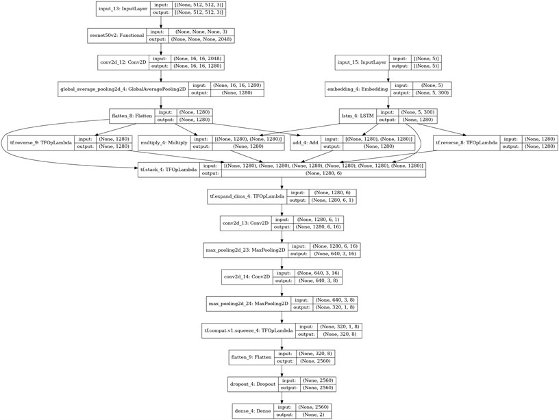
We propose a new method for fusing features, which work as follows: we form a matrix from original feature vectors, reversed feature vectors, and summed as well as multiplied vectors (using the same notation as in 2.3.1. chapter):
After formatting matrix , we apply 2 convolutional layers with 16 and 8 filters, both with kernel size equal to 3×3 and max pooling layers. The resulting feature maps are flattened and then passed to a dense fully connected layer to calculate the class distribution probabilities (Fig. 13).
Fig. 13Architecture with custom matrix based on ResNet50V2 and LSTM backbones
This particular feature fusion strategy serves as an enhancement of the network with some of the possible interactions between different types of features. Using the signal together with its reversed copy and blending them by different operations enrich the model with feature interactions. In addition to this, convolutional kernels then serve as an additional interaction learning tool: a small number of learnable parameters in convolutional kernels serves as a kind of regularization (as compared to the use of a densely connected layer) on top of that.
3.3.3. Feature importance weights
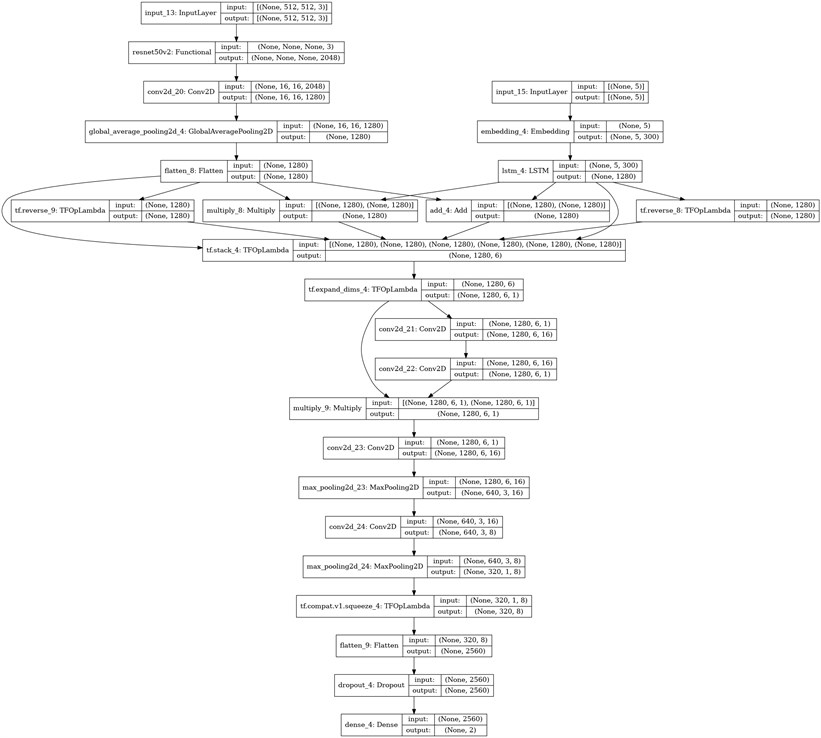
This idea is based on 2.3.2. chapter operations, but in this case, we let the model choose which feature vectors are the most important. To achieve this behavior, once the matrix is constructed, a convolutional layer (3×3 kernel size) with 16 filters and a convolutional layer (1×1 kernel size) with 1 filter is applied. The resulting feature maps are processed with a Sigmoid activation function and then the resulting values are multiplied with the same matrix (Fig. 14). Note that the sigmoid values are in the interval [0; 1], so this activation enables the deactivation of unimportant features.
Fig. 14Architecture with custom matrix and weights based on ResNet50V2 and LSTM backbones
4. Analysis
The VQA-2019 Med [1] dataset was used for what follows. Only questions whose answers can be 'yes' or 'no' were considered. Other types of answers had a very small number of data points, and thus were removed for analysis. In total, there were 1560 questions-answer pairs, 24 unique words (after data cleaning), and 33 unique questions. To obtain an accuracy estimate of each model, 5-fold cross-validation was used: in each fold, there were 305 test images and 1218 train images. In Fig. 15 some examples of image-question pairs are provided.
Fig. 15Examples of image-question pairs used in the work [1]
![Examples of image-question pairs used in the work [1]](https://static-01.extrica.com/articles/22737/22737-img16.jpg)
The following is the list of parameters and architectural choices that were considered in this work:
1) word embeddings [21] pre-trained on Wikipedia texts were used. Each vector had a length of 300;
2) the images had a 512×512 shape; using smaller images destroys valuable information;
3) to avoid overfitting shift, rotation, contrast, blur, and distortion augmentations were added to flow;
4) the Adam optimization algorithm was used to train all networks, learning rate equal to 0.00002, batch size equal to 8;
5) for each fusion idea (addition, concatenation, custom matrix, custom matrix with weights), 4 models were trained: LSTM together with ResNet or EfficientNet backbones, and RNN, with ResNet backbones or EfficienNet backbones.
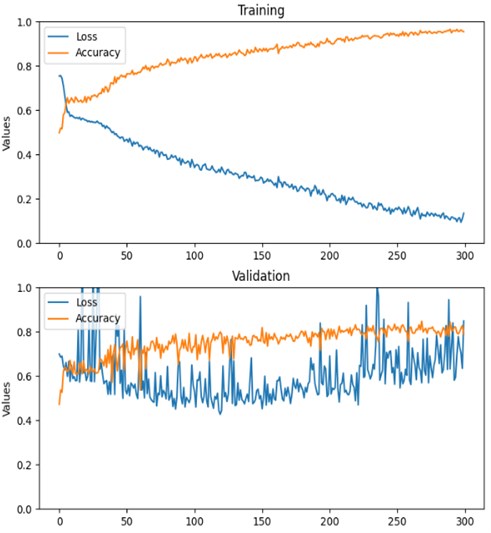
In Table 1 we provide results with the corresponding best backbone combinations, while in Fig. 18 the best model training process can be found.
Table 1Models’ benchmarks
Question category | Fusion type | |||
Addition | Concatenation | Custom matrix | Custom matrix with weights | |
Backbones | LSTM, EfficientNetB0 | LSTM, ResNet50V2 | LSTM, ResNet50V2 | LSTM, EfficientNetB0 |
Image normality | 77,41 % | 80,64 % | 80,64 % | 78,49 % |
Anomalies in image | 74,50 % | 74,51 % | 76,47 % | 72,54 % |
Image type | 90,02 % | 91,47 % | 92,91 % | 91,86 % |
Contrast usage | 73,70 % | 72,32 % | 76,60 % | 75,68 % |
Overall average | 81,91 % | 82,24 % | 84,80 % | 83,65 % |
As can be seen from Fig. 16 model after 150 epochs face an overfitting problem, but since we use the best model weights and not the last model weights, we train models in our experiments on more epochs to be sure that underfitting will not occur. From Table 1 can be seen that for all fusion ideas the easiest category was image type: learning visual features for image type classification is a more straightforward task than detecting contrast liquid, different types of anomalies or identifying image normality.
Also, all backbones were better with long-short term memory networks: we face this situation because of the vanishing or exploding gradients, since, as mentioned in the methods chapter, these models protect gradients in a more trustworthy way than recurrent neural networks. The highest results were achieved with the ResNet50V2 backbone and the custom matrix fusion option. We believe that a convolutional neural network with more parameters (compared to EfficientNetB0) helps to keep semantic information in a more reliable way, which leads to the situation that further convolutional layers can further highlight this information in a more accurate way than, for example, densely connected layers whose input are concatenated or summed visual and text features. Talking about evaluations, experiments have shown that the best architecture used a fusion mechanism constructed by a feature matrix; second one was the same matrix idea but with custom weights, and less accurate architectures used addition and concatenation operations for combining text and image features. Note that the best model had 55 214 762 parameters, while the summation, concatenation, and additional weights ideas had 56 005 814, 33 468 342, and 55 214 939 corresponding parameters. This insight highlights the model’s ability to solve problems in a more efficient way than other approaches (summation, additional weights adding). However, the concatenation fusion option had fewer parameters, but, as mentioned below, by combining image and text features independently, we lose too much information between the connections of different features, and a smaller number of parameters (and slightly faster inference) do not overestimate the accuracy of the model.
Fig. 16Training history of LSTM (ResNet50V2 backbone) with custom matrix fusion
5. Conclusions
In this paper, the authors proposed a feature fusion for different language and image domains. The method enables to retain larger amount of information about possible interactions between different types of features without increasing the number of unknown parameters.
Research has shown that the proposed fusion method which formats the matrix following convolution operations delivers the best results in all the question categories with an average accuracy equal to 84,80 %. When we applied additional weights for the custom matrix, results did not improve, but this idea was still better with an average accuracy equal to 83.65 % than concatenation or addition with corresponding accuracies equal to 82,24 % and 81,91 %. Also, experiments showed that in each fusion option, the best textual information calculation model was LSTM, while for digital images, the best model had a ResNet backbone.
As a future study, the authors intend to extend the feature fusion strategy to include an additional attention mechanism loop, which might further improve the accuracy of the models.
References
-
Asma Ben Abacha, Sadid A. Hasan, Vivek Datla, Joey Liu, Dina Demner-Fushman, and H. Müller, “VQA-Med: overview of the medical visual question answering task at ImageCLEF 2019,” in CLEF 2019 Working Notes, 2019.
-
D. Sharma, S. Purushotham, and C. K. Reddy, “MedFuseNet: An attention-based multimodal deep learning model for visual question answering in the medical domain,” Springer Science and Business Media LLC, Scientific Reports, Dec. 2021.
-
B. Duke and G. W. Taylor, “Generalized Hadamard-product fusion operators for visual question answering,” in 15th Canadian Conference on Computer and Robot Vision, pp. 39–46, 2018, https://doi.org/10.48550/arxiv.1803.09374
-
Xin Yan, Lin Li, Chulin Xie, Jun Xiao, and Lin Gu, “Zhejiang University at ImageCLEF 2019 visual question answering in the medical domain,” in CLEF 2019 Working Notes, 2019.
-
A. Abacha, S. Gayen, J. Lau, S. Rajaraman, and D. Demner-Fushman, “NLM at ImageCLEF 2018 Visual Question Answering in the Medical Domain,” in CLEF 2018 Working Notes, 2018.
-
M. Sarrouti, “NLM at VQA-Med 2020: visual question answering and generation in the medical domain,” in CLEF 2020 Working Notes, 2020.
-
Y. Zhou, X. Kang, and F. Ren, “Employing inception-resnet-v2 and Bi-LSTM for medical domain visual question answering,” in CLEF 2018 Working Notes, 2018.
-
T. Mikolov, K. Chen, G. Corrado, and J. Dean, “Efficient estimation of word representations in vector space,” in International Conference on Learning Representations, 2013, https://doi.org/10.48550/arxiv.1301.3781
-
L. T. K. Nguyen, H.-H. Chung, K. V. Tuliao, and T. M. Y. Lin, “Using XGBoost and skip-gram model to predict online review popularity,” SAGE Open, Vol. 10, No. 4, p. 215824402098331, Oct. 2020, https://doi.org/10.1177/2158244020983316
-
P. Liu, X. Qiu, and X. Huang, “Recurrent neural network for text classification with multi-task learning,” in 25th International Joint Conference on Artificial Intelligence IJCAI-16, 2016, https://doi.org/10.48550/arxiv.1605.05101
-
S. Song, H. Huang, and T. Ruan, “Abstractive text summarization using LSTM-CNN based deep learning,” Multimedia Tools and Applications, Vol. 78, No. 1, pp. 857–875, Jan. 2019, https://doi.org/10.1007/s11042-018-5749-3
-
J. Peng, A. Kimmig, J. Wang, X. Liu, Z. Niu, and J. Ovtcharova, “Dual-stage attention-based long-short-term memory neural networks for energy demand prediction,” Energy and Buildings, Vol. 249, p. 111211, Oct. 2021, https://doi.org/10.1016/j.enbuild.2021.111211
-
K. He, X. Zhang, S. Ren, and J. Sun, “Deep residual learning for image recognition,” in Computer Vision and Pattern Recognition, 2015, https://doi.org/10.48550/arxiv.1512.03385
-
E. Rezende, G. Ruppert, T. Carvalho, F. Ramos, and P. de Geus, “Malicious software classification using transfer learning of ResNet-50 deep neural network,” in 16th IEEE International Conference on Machine Learning and Applications (ICMLA), Dec. 2017, https://doi.org/10.1109/icmla.2017.00-19
-
K. He, X. Zhang, S. Ren, and J. Sun, “Identity mappings in deep residual networks,” in Computer Vision – ECCV 2016, pp. 630–645, 2016, https://doi.org/10.1007/978-3-319-46493-0_38
-
M. Tan and Q. V. Le, “EfficientNet: rethinking model scaling for convolutional neural networks,” 36th International Conference on Machine Learning, 2019, https://doi.org/10.48550/arxiv.1905.11946
-
S. Gang, N. Fabrice, D. Chung, and J. Lee, “Character recognition of components mounted on printed circuit board using deep learning,” Sensors, Vol. 21, No. 9, p. 2921, Apr. 2021, https://doi.org/10.3390/s21092921
-
M. Sandler, A. Howard, M. Zhu, A. Zhmoginov, and L.-C. Chen, “MobileNetV2: inverted residuals and linear bottlenecks,” in Computer Vision and Pattern Recognition, 2018, https://doi.org/10.48550/arxiv.1801.04381
-
P. Ramachandran, B. Zoph, and Q. V. Le, “Searching for Activation Functions,” in Computer Vision and Pattern Recognition, 2017, https://doi.org/10.48550/arxiv.1710.05941
-
J. Hu, L. Shen, S. Albanie, G. Sun, and E. Wu, “Squeeze-and-excitation networks,” in Computer Vision and Pattern Recognition, 2017, https://doi.org/10.48550/arxiv.1709.01507
-
T. Mikolov, E. Grave, P. Bojanowski, C. Puhrsch, and A. Joulin, “Advances in pre-training distributed word representations,” in Proceedings of the Eleventh International Conference on Language Resources and Evaluation, 2017, https://doi.org/10.48550/arxiv.1712.09405
About this article

