Improved algorithm for a system with different stiffness for positive and negative displacements

Ragulskis, K.; Spruogis, B.; Matuliauskas, A.; Mištinas, V.; Ragulskis, L.

doi:10.21595/mme.2022.22748

Mathematical Models in Engineering

Browse Journal

Submit article

Published: 30 June 2022

Check for updates

Improved algorithm for a system with different stiffness for positive and negative displacements

K. Ragulskis¹

B. Spruogis²

A. Matuliauskas³

V. Mištinas⁴

L. Ragulskis⁵

¹Kaunas University of Technology, K. Donelaičio str. 73, LT-44249, Kaunas, Lithuania

^{2, 3, 4}Department of Mobile Machinery and Railway Transport, Faculty of Transport Engineering, Vilnius Gediminas Technical University, Plytinės str. 27, LT-10105, Vilnius, Lithuania

⁵Department of Systems Analysis, Faculty of Informatics, Vytautas Magnus University, Vileikos str. 8, LT-44404, Kaunas, Lithuania

Corresponding Author:

K. Ragulskis

Cite the article Download PDF

Downloads 326

Abstract

In the process of investigation of dynamics of elements of robots, systems with different values of stiffness for positive and negative displacements play an important role. This change of the value of stiffness has an effect to the results of numerical calculation of dynamics of the system. For more precise investigation of dynamics a special numerical procedure is proposed in the paper. Numerical results for two values of time steps: large and medium ones, are presented for two cases: without application of the proposed procedure and with application of it. Comparison of the presented results indicates advantages of the proposed numerical procedure.

1. Introduction

In the process of investigation of dynamics of elements of robots, systems with different values of stiffness for positive and negative displacements play an important role. This change of the value of stiffness has an effect to the results of numerical calculation of dynamics of the system.

For more precise investigation of dynamics a special numerical procedure is proposed in the paper. Numerical results for two values of time steps: large and medium ones, are presented for two cases: without application of the proposed procedure and with application of it.

Comparison of the presented results indicates advantages of the proposed numerical procedure.

Resonances in nonlinear systems are described in [1]. Systems with impacts are investigated in [2]. Stabilisation of dynamical systems is presented in [3]. Impacts in vibrating systems are investigated in [4]. Periodic orbits are analysed in [5]. Vibro-impact energy sink is investigated in [6]. Particle impact with a wall is presented in [7]. Frequencies of a multibody system are analysed in [8]. Pendulum and its dynamics are investigated in [9]. Piecewise linearity is analysed in [10]. Resonant zones are investigated in [11]. Sommerfeld effect is presented in [12]. Isolated resonances are investigated in [13].

First the model of the system with a single degree of freedom and harmonic excitation is described. Then the proposed procedure for improved calculation of dynamics is presented. Graphical results without application of the proposed procedure and with it are presented and mutually compared.

2. Model of the system with different values of stiffness for positive and negative displacements

The investigated system has a single degree of freedom and is described by the following differential equation:

1

\ddot{x} + 2 h \dot{x} + p^{2} x = - f s i n ω t,

where $x$ is the displacement of the system, $h$ is the coefficient of viscous damping, $p^{2}$ is the nonlinear coefficient of stiffness, $f$ is the amplitude of harmonic excitation, $ω$ is the frequency of harmonic excitation, $t$ is the time and the upper dot denotes differentiation with respect to it.

It is assumed that the nonlinear stiffness has the following form:

2

p^{2} = \{\begin{array}{l} p_{2}^{2}, x > 0, \\ p_{1}^{2}, e l s e w h e r e, \end{array}

where $p_{1}$ and $p_{2}$ are constant values.

Further the force of stiffness is denoted as:

3

P = p^{2} x .

3. Improved procedure for calculation of dynamics of the system with different values of stiffness for positive and negative displacements

Further the following notation is used: $T$ denotes the time step, the subscript $0$ denotes the value at the beginning of a time step and the subscript $T$ denotes the value at the end of a time step.

It is assumed that:

4

p^{2} = \{\begin{array}{l} p_{2}^{2}, (x > 0) \lor ((x = 0) & (\dot{x} > 0)), \\ p_{1}^{2}, e l s e w h e r e . \end{array}

If the following conditions are satisfied:

5

x_{T} > 0,

and:

6

x_{0} < 0,

or if the following conditions are satisfied:

7

x_{T} < 0,

and:

8

x_{0} > 0,

then the reduced time step is used in the process of calculations:

9

T_{r} = - \frac{x_{0}}{x_{T} - x_{0}} T .

Then it is assumed that:

10

x_{T_{r}} = 0,

11

{\dot{x}}_{T_{r}} = {\dot{x}}_{0} + ({\dot{x}}_{T} - {\dot{x}}_{0}) \frac{T_{r}}{T},

12

{\ddot{x}}_{T_{r}} = {\ddot{x}}_{0} + ({\ddot{x}}_{T} - {\ddot{x}}_{0}) \frac{T_{r}}{T} .

4. Investigation of dynamics of the system with different values of stiffness for positive and negative displacements

The following parameters of the investigated system with different values of stiffness for positive and negative displacements were assumed:

13

ω = 1, f = 1, h = 0.1, p_{1} = 1, p_{2} = 2 .

Zero initial conditions were assumed:

14

x (0) = 0, \dot{x} (0) = 0 .

Results for two values of a time step are presented: large time step:

15

T = \frac{2 π}{ω 40},

and medium time step:

16

T = \frac{2 π}{ω 80} .

4.1. Results of investigation of the system with different values of stiffness for positive and negative displacements for large time step

4.1.1. Conventional procedure for calculation of dynamics

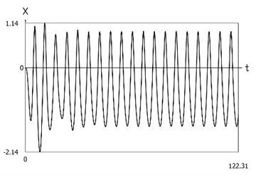
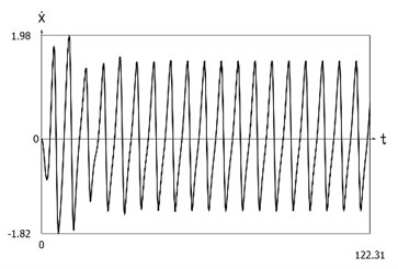
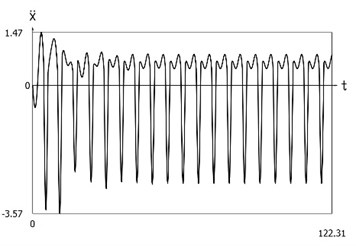
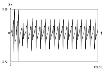
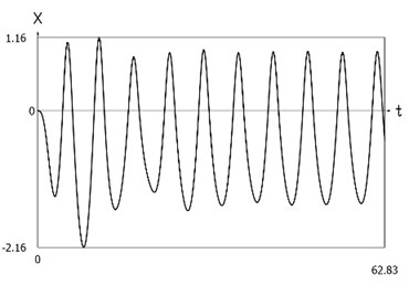
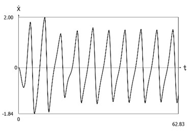
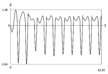
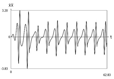
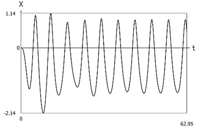
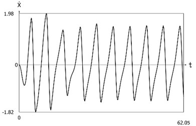
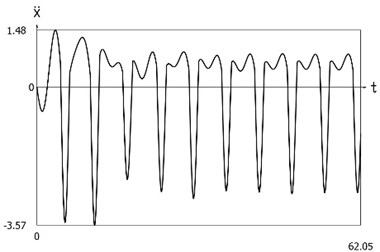
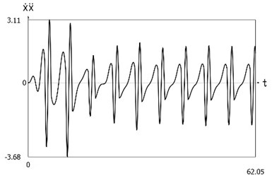
Displacement, velocity, acceleration, and velocity multiplied by acceleration as functions of time are presented in Fig. 1.

Fig. 1Dynamics of the system with different values of stiffness for positive and negative displacements when ω=1, f= 1, h= 0.1, p1= 1, p2= 2

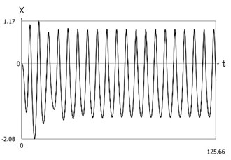
a) Displacement as function of time

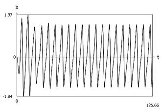
b) Velocity as function of time

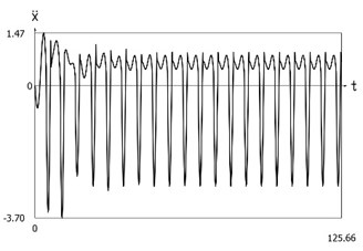
c) Acceleration as function of time

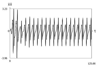
d) Velocity multiplied by acceleration as function of time

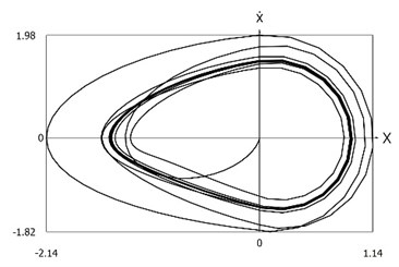
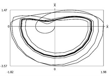
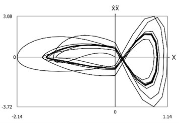
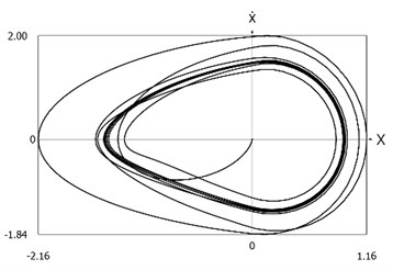
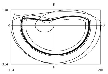
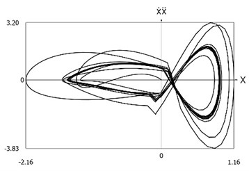
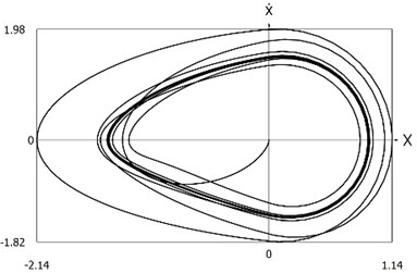
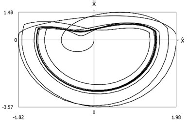
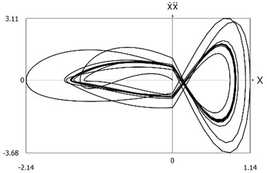
Phase trajectories of motion of the investigated system are presented in Fig. 2.

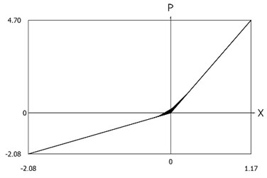
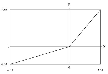
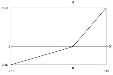
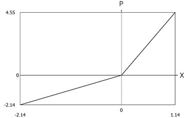
Force of stiffness as function of displacement is shown in Fig. 3.

Fig. 2Phase trajectories of the system with different values of stiffness for positive and negative displacements when ω=1, f= 1, h= 0.1, p1= 1, p2= 2

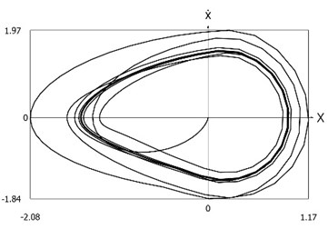
a) Velocity as function of displacement

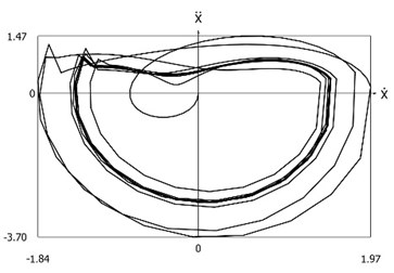
b) Acceleration as function of velocity

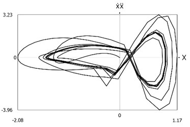
c) Velocity multiplied by acceleration as function of displacement

Fig. 3Force of stiffness as function of displacement of the system with different values of stiffness for positive and negative displacements when ω=1, f= 1, h= 0.1, p1= 1, p2= 2

Force of stiffness as function of displacement of the system with different values of stiffness for positive and negative displacements when ω=1, f= 1, h= 0.1, p1= 1, p2= 2

4.1.2. Improved procedure for calculation of dynamics

Displacement, velocity, acceleration, and velocity multiplied by acceleration as functions of time are presented in Fig. 4.

Phase trajectories of motion of the investigated system are presented in Fig. 5.

Force of stiffness as function of displacement is shown in Fig. 6.

From the presented results it is seen that the improved procedure for calculation of dynamics has advantages, which are seen from the comparison of corresponding graphical representations. This is especially evident from the comparison of corresponding drawings involving accelerations as well as from the comparison of representations of force of stiffness as function of displacement in the vicinity of the origin of the coordinate system.

Fig. 4Dynamics of the system with different values of stiffness for positive and negative displacements when ω=1, f= 1, h= 0.1, p1= 1, p2= 2

a) Displacement as function of time

b) Velocity as function of time

c) Acceleration as function of time

d) Velocity multiplied by acceleration as function of time

Fig. 5Phase trajectories of the system with different values of stiffness for positive and negative displacements when ω=1, f= 1, h= 0.1, p1= 1, p2= 2

a) Velocity as function of displacement

b) Acceleration as function of velocity

c) Velocity multiplied by acceleration as function of displacement

Fig. 6Force of stiffness as function of displacement of the system with different values of stiffness for positive and negative displacements when ω=1, f= 1, h= 0.1, p1= 1, p2= 2

4.2. Results of investigation of the system with different values of stiffness for positive and negative displacements for medium time step

4.2.1. Conventional procedure for calculation of dynamics

Displacement, velocity, acceleration, and velocity multiplied by acceleration as functions of time are presented in Fig. 7.

Fig. 7Dynamics of the system with different values of stiffness for positive and negative displacements when ω=1, f= 1, h= 0.1, p1= 1, p2= 2

a) Displacement as function of time

b) Velocity as function of time

c) Acceleration as function of time

d) Velocity multiplied by acceleration as function of time

Phase trajectories of motion of the investigated system are presented in Fig. 8.

Force of stiffness as function of displacement is shown in Fig. 9.

Fig. 8Phase trajectories of the system with different values of stiffness for positive and negative displacements when ω=1, f= 1, h= 0.1, p1= 1, p2= 2

a) Velocity as function of displacement

b) Acceleration as function of velocity

c) Velocity multiplied by acceleration as function of displacement

Fig. 9Force of stiffness as function of displacement of the system with different values of stiffness for positive and negative displacements when ω=1, f= 1, h= 0.1, p1= 1, p2= 2

4.2.2. Improved procedure for calculation of dynamics

Displacement, velocity, acceleration, and velocity multiplied by acceleration as functions of time are presented in Fig. 10.

Phase trajectories of motion of the investigated system are presented in Fig. 11.

Force of stiffness as function of displacement is shown in Fig. 12.

From the presented results it is seen that the improved procedure for calculation of dynamics has advantages, which are seen from the comparison of corresponding graphical representations. This is especially evident from the comparison of corresponding drawings involving accelerations as well as from the comparison of representations of force of stiffness as function of displacement in the vicinity of the origin of the coordinate system.

The presented graphical representations show the advantages of the improved procedure for calculation of dynamics of the system with different values of stiffness for positive and negative displacements.

Fig. 10Dynamics of the system with different values of stiffness for positive and negative displacements when ω=1, f= 1, h= 0.1, p1= 1, p2= 2

a) Displacement as function of time

b) Velocity as function of time

c) Acceleration as function of time

d) Velocity multiplied by acceleration as function of time

Fig. 11Phase trajectories of the system with different values of stiffness for positive and negative displacements when ω=1, f= 1, h= 0.1, p1= 1, p2= 2

a) Velocity as function of displacement

b) Acceleration as function of velocity

c) Velocity multiplied by acceleration as function of displacement

Fig. 12Force of stiffness as function of displacement of the system with different values of stiffness for positive and negative displacements when ω=1, f= 1, h= 0.1, p1= 1, p2= 2

5. Conclusions

Systems with different values of stiffness for positive and negative displacements are important in engineering applications. This change of the value of stiffness has an effect to the results of numerical calculation of dynamics of the system. For more precise investigation of dynamics a special numerical procedure is proposed in the paper. Numerical results for two values of time steps are presented without application of the proposed procedure and with application of it.

Displacement, velocity, acceleration, and velocity multiplied by acceleration as functions of time are investigated. Also phase trajectories of motion of the investigated system are presented. Force of stiffness as function of displacement is calculated and graphically represented.

From the presented results it is seen that the improved procedure for calculation of dynamics has advantages, which are seen from the comparison of corresponding graphical representations. This is especially evident from the comparison of corresponding drawings involving accelerations as well as from the comparison of representations of force of stiffness as function of displacement in the vicinity of the origin of the coordinate system. The presented graphical representations show the advantages of the improved procedure for calculation of dynamics of the system with different values of stiffness for positive and negative displacements.

The results of the performed investigation are applied in the process of design of elements of robots.

References

W. Wedig, “New resonances and velocity jumps in nonlinear road-vehicle dynamics,” Procedia IUTAM, Vol. 19, pp. 209–218, 2016.

Publisher
T. Li, E. Gourc, S. Seguy, and A. Berlioz, “Dynamics of two vibro-impact nonlinear energy sinks in parallel under periodic and transient excitations,” International Journal of Non-Linear Mechanics, Vol. 90, pp. 100–110, Apr. 2017, https://doi.org/10.1016/j.ijnonlinmec.2017.01.010

Publisher
V. A. Zaitsev, “Global asymptotic stabilization of periodic nonlinear systems with stable free dynamics,” Systems and Control Letters, Vol. 91, pp. 7–13, May 2016, https://doi.org/10.1016/j.sysconle.2016.01.004

Publisher
H. Dankowicz and E. Fotsch, “On the analysis of chatter in mechanical systems with impacts,” Procedia IUTAM, Vol. 20, pp. 18–25, 2017, https://doi.org/10.1016/j.piutam.2017.03.004

Publisher
S. Spedicato and G. Notarstefano, “An optimal control approach to the design of periodic orbits for mechanical systems with impacts,” Nonlinear Analysis: Hybrid Systems, Vol. 23, pp. 111–121, 2017, https://doi.org/10.48550/arxiv.1702.04544

Publisher
W. Li, N. E. Wierschem, X. Li, and T. Yang, “On the energy transfer mechanism of the single-sided vibro-impact nonlinear energy sink,” Journal of Sound and Vibration, Vol. 437, pp. 166–179, Dec. 2018, https://doi.org/10.1016/j.jsv.2018.08.057

Publisher
J. S. Marshall, “Modeling and sensitivity analysis of particle impact with a wall with integrated damping mechanisms,” Powder Technology, Vol. 339, pp. 17–24, Nov. 2018, https://doi.org/10.1016/j.powtec.2018.07.097

Publisher
E. Salahshoor, S. Ebrahimi, and Y. Zhang, “Frequency analysis of a typical planar flexible multibody system with joint clearances,” Mechanism and Machine Theory, Vol. 126, pp. 429–456, Aug. 2018, https://doi.org/10.1016/j.mechmachtheory.2018.04.027

Publisher
U. Starossek, “Forced response of low-frequency pendulum mechanism,” Mechanism and Machine Theory, Vol. 99, pp. 207–216, May 2016, https://doi.org/10.1016/j.mechmachtheory.2016.01.004

Publisher
S. Wang, L. Hua, C. Yang, Y.O. Zhang, and X. Tan, “Nonlinear vibrations of a piecewise-linear quarter-car truck model by incremental harmonic balance method,” Nonlinear Dynamics, Vol. 92, No. 4, pp. 1719–1732, Jun. 2018, https://doi.org/10.1007/s11071-018-4157-6

Publisher
P. Alevras, S. Theodossiades, and H. Rahnejat, “On the dynamics of a nonlinear energy harvester with multiple resonant zones,” Nonlinear Dynamics, Vol. 92, No. 3, pp. 1271–1286, May 2018, https://doi.org/10.1007/s11071-018-4124-2

Publisher
A. Sinha, S. K. Bharti, A. K. Samantaray, G. Chakraborty, and R. Bhattacharyya, “Sommerfeld effect in an oscillator with a reciprocating mass,” Nonlinear Dynamics, Vol. 93, No. 3, pp. 1719–1739, Aug. 2018, https://doi.org/10.1007/s11071-018-4287-x

Publisher
G. Habib, G. I. Cirillo, and G. Kerschen, “Isolated resonances and nonlinear damping,” Nonlinear Dynamics, Vol. 93, No. 3, pp. 979–994, Aug. 2018, https://doi.org/10.1007/s11071-018-4240-z

Publisher

About this article

Received

06 May 2022

Accepted

24 June 2022

Published

30 June 2022

DOI

https://doi.org/10.21595/mme.2022.22748

Keywords

different values of stiffness

harmonic excitation

transient processes

This is an open access article distributed under the Creative Commons Attribution License, which permits unrestricted use, distribution, and reproduction in any medium, provided the original work is properly cited.

Previous article in issue Previous

Research article

2024 01 21

Study on the effect of rolling mill dynamic stiffness on coupled vibration of hydraulic machine

Lidong Wang, Peng Hou, Shen Wang, Chengzhen Wang, Xiaoqiang Yan, Xiaoling Wang

Research article

2023 12 30

Modelling and dynamic behaviours of a high-contact-ratio spur-gear system considering rough surface

Zhenbang Cheng, Yu Zhou, Zhengyu Liu

Research article

2020 02 15

Dynamic simulation analysis of spur gear space driven system with large inertia load

Chao Li, Jianfeng Ma, Xuehao Yin, Hongbin Yang

Research article

2018 12 31

Improvement of vibration isolation performance of QZS platform in chaotic interval based on damping increase control method

Peicheng Shi, Peilei Shi, Gaofa Nie, Ye Tang, Daoyuan Pan

K. Ragulskis, B. Spruogis, A. Matuliauskas, V. Mištinas, and L. Ragulskis, “Improved algorithm for a system with different stiffness for positive and negative displacements,” Mathematical Models in Engineering, Vol. 8, No. 2, pp. 72–81, Jun. 2022, https://doi.org/10.21595/mme.2022.22748

Copy Extrica

Copied to clipboard!

TY  - JOUR
DO  - 10.21595/mme.2022.22748
UR  - https://doi.org/10.21595/mme.2022.22748
TI  - Improved algorithm for a system with different stiffness for positive and negative displacements
T2  - Mathematical Models in Engineering
AU  - Ragulskis, K.
AU  - Spruogis, B.
AU  - Matuliauskas, A.
AU  - Mištinas, V.
AU  - Ragulskis, L.
PY  - 2022
DA  - 2022/06/30
PB  - JVE International Ltd.
SP  - 72-81
VL  - 8
IS  - 2
SN  - 2351-5279
SN  - 2424-4627
ER  - 

Copy Ris

Copied to clipboard!

@article{Ragulskis_2022,
	doi = {10.21595/mme.2022.22748},
	url = {https://doi.org/10.21595/mme.2022.22748},
	year = 2022,
	month = {jun},
	publisher = {{JVE} International Ltd.},
	volume = {8},
	number = {2},
	pages = {72--81},
	author = {K. Ragulskis and B. Spruogis and A. Matuliauskas and V. Mi{\v{s}}tinas and L. Ragulskis},
	title = {Improved algorithm for a system with different stiffness for positive and negative displacements},
	journal = {Mathematical Models in Engineering}
}

Copy Bibtex

Copied to clipboard!

[1]K. Ragulskis, B. Spruogis, A. Matuliauskas, V. Mištinas, and L. Ragulskis, “Improved algorithm for a system with different stiffness for positive and negative displacements,” Mathematical Models in Engineering, vol. 8, no. 2, pp. 72–81, Jun. 2022, doi: 10.21595/mme.2022.22748.

Copy IEEE

Copied to clipboard!

Ragulskis, K., B. Spruogis, A. Matuliauskas, V. Mištinas, and L. Ragulskis. “Improved Algorithm for a System with Different Stiffness for Positive and Negative Displacements.” Mathematical Models in Engineering 8, no. 2 (June 26, 2022): 72–81. https://doi.org/10.21595/mme.2022.22748.

Copy Chicago

Copied to clipboard!

Improved algorithm for a system with different stiffness for positive and negative displacements

Abstract

1. Introduction

2. Model of the system with different values of stiffness for positive and negative displacements

3. Improved procedure for calculation of dynamics of the system with different values of stiffness for positive and negative displacements

4. Investigation of dynamics of the system with different values of stiffness for positive and negative displacements

4.1. Results of investigation of the system with different values of stiffness for positive and negative displacements for large time step

4.1.1. Conventional procedure for calculation of dynamics

4.1.2. Improved procedure for calculation of dynamics

4.2. Results of investigation of the system with different values of stiffness for positive and negative displacements for medium time step

4.2.1. Conventional procedure for calculation of dynamics

4.2.2. Improved procedure for calculation of dynamics

5. Conclusions

References

About this article

Related Articles