Abstract
The complex boundary modeling required for simulating composite materials was applied to a broad range of problems, including surface overlap and gap. A novel method for the simultaneous fitting of adjacent spline surfaces based on a distance field has been devised. The fitting method for spline surfaces was constructed using offline spline surface, facet simplification, and residual solid reconstruction. The distance field-based approach of simultaneous fitting of neighboring spline surfaces included producing a distance field for a spline surface and then applying that distance field to nearby spline surfaces. There would be junction and separation issues if neighboring spline surfaces were fitted individually. By simultaneously fitting the nearby spline surfaces with the aid of the equivalence surface of the distance field, it was feasible to avoid overlap and gap.
1. Introduction
There are two types of surfaces in CAD systems: analytic surfaces and free-form surfaces [1]. Analytic surfaces include planes, columns, cones, spheres, and torus were generally used to represent simple, regular model surfaces; free-form surfaces, which are relatively complex surfaces in a model, are generally represented by B-Splines and Non-Uniform Rational B-Splines (NURBS) method to represent the relatively complex surfaces in the model [2-3].
The distance field-based simultaneous fitting algorithm for adjacent spline surfaces was designed to synchronize the free spline surfaces in the CAD model, and its basic principle was to build a set of simple planar slices (triangular slices were used in this paper) to fit the CAD model's spline surfaces [4]. The spline surfaces in the model were found, and the transition area was segmented; the distance field was then constructed; and lastly, the equivalency surface was extracted to provide a close approximation of the spline surfaces.
The algorithm consists of three parts: the discretization of the spline surface, the facet simplification and the remaining solid reconstruction. According to the B-Rep representation adopted by the CAD model, and the characteristics of the radiation transport calculation model [5]. The design and implementation of the algorithm in this paper mainly considers the following three principles.
(1) After the sample surface processing, the intersection interface between adjacent entities of the co-sample surface remains consistent without gaps or overlaps. If a single entity is fitted separately, the gaps and overlaps between the adjacent entities of the co-sample surface will lead to errors in the subsequent Monte Carlo (MC) calculation [6].
(2) The number of facets produced after the sample surface is discretized can be controlled. On the one hand, if the shape of the spline surface is complex, the number of facets generated after the extraction of the equivalent surface is large, which reduces the computational speed. On the other hand, after the CAD model is converted into a radiation transport calculation model, the MC calculation program has restrictions on the length of the expressions described by its grid elements, in which the length of the expressions of the MCNP4C grid elements should be less than 1000 characters [7].
(3) The CAD model boundary satisfies the principle of closure. No gaps or overlaps can be created between the combinations of plane slices and flat slices of the fitted sample surfaces and the remaining adjacent surfaces of the original model to provide accurate geometric data and topological information for the remaining entities [8].
In this paper, a simultaneous fitting algorithm for multi-strip surfaces based on distance fields is proposed. First, the transition region boundary delineation and the multi-strip surface discretization are performed simultaneously. Then, the discretized surface pieces are simplified and the number of pieces is reasonably controlled. Finally, the remaining entities are reconstructed. In the following, the basic principle and implementation of the algorithm are described in detail from three aspects, namely, the discretization of the spline surface, the simplification of the face slices and the reconstruction of the remaining entities.
2. Spline surface discretization
Surface discretization, also known as surface meshing, was first proposed by Catmull [9], and applied to the field of computer graphics display, and was a relatively mature technique in computer graphics. The goal was to discretize surfaces into pixel-level planar slices for displaying and rendering surfaces in a computer. Surface discretization has also been widely studied and applied in CAD, CAM, virtual reality and virtual simulation, computer animation, and other fields. For example, in finite element analysis, surface discretization was the premise and basis of finite element meshing, which directly affected the quality of finite element mesh and the accuracy of subsequent calculations; and in virtual reality and virtual simulation, complex surfaces in solids were usually discretized into a series of planar slices, and then the Boolean intersection operation between planar slices was used to achieve rapid detection of collision information between entities.
3. Distance field generation
Distance fields were one of the basic graphical representations in computer graphics, which were first applied by researchers in areas such as body drawing and offset surface creation, and later developed in areas such as computer animation and solid modeling [10]. Usually, distance fields were divided into unsigned distance fields and signed distance fields, and signed distance fields were often used in graphics. The surface of the solid was closed, and positive and negative signs can be used to discriminate whether the discrete points were located inside or outside the solid.
The unsigned and signed distance fields were defined as follows [11].
Suppose a point in any set of space, the unsigned function of the distance field from that point to the nearest point of the set can be expressed as:
Based on Eq. (1), assume that is a closed surface in the set , then the signed distance field from any point in to the nearest point on the surface can be expressed as:
where:
The value of the distance was calculated as the shortest distance from each discrete point in the field to the spline surface. Specifically, this was done by first finding the projection point of the discrete point on the spline surface, i.e., the point on the spline surface closest to the discrete point, and then calculating the distance between the two points of the discrete point and its projection point. Since for the model with closed smooth surface, the direction of the normal vector of the surface pointed to the outside of the object. Therefore, the sign of the distance field was calculated by determining the angle between the normal vector of the projection point on the sample surface, and the vector consisting of the projection point and the discrete point. If it was less than 90°, the distance sign of the point was "+"; if it was greater than 90°, the distance sign of the point was "–". An example of distance calculation for three different locations of discrete points was shown in Fig.1, where points , , and denoted points in the distance field.Points , , and denoted the mapping points of points , , and on the spline surface, i.e., the nearest points on the spline surface to points , , and .
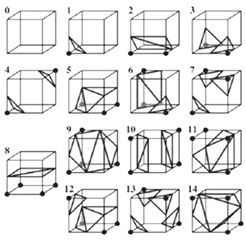
Equivalent surface is a plane or surface composed of points with the same attribute value in the 3D data field [12]. The classical method for equivalence surface extraction in 3D regular data fields was the Marching Cubes algorithm proposed by Lorensen and CIine [13] in 1987. The first step was to determine the voxels containing the isosurface and the corresponding edges. The voxel in the MC algorithm was composed of eight vertices of the voxel with four data points in each of the two adjacent layers of the distance field, as shown in Fig.2. After considering complementary symmetry and rotational symmetry, these 256 kinds can be simplified into fifteen patterns, as shown in Fig. 3.
Fig. 1Distance calculation
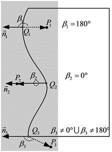
Fig. 2Construction of voxel
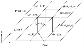
Fig. 3Fifteen modes
The second step was to find the intersection of isosurface and voxel boundary. When the voxel was very small, it could be assumed that the function value varies linearly along the boundary of the voxel, therefore, according to this assumption of the Marching Cubes algorithm, linear interpolation could be used to calculate the intersection of the equivalence surface and the voxel edge. The linear interpolation calculation formula was:
where represented the coordinates of the requested intersection, and represented the coordinates of the two vertices of the voxel edges, and represented the distance values of the two vertices in the distance field, and isovalue represented the threshold value of the extracted isovalue surface.
4. Simplification of spline surfaces
In order to meet the accuracy requirements, for the sample surface with complex geometry, the sample surface discretization using the equivalence surface extraction method generated a large number of plane slices, which leaded to an excessive number of unstructured meshes generated later and a reduced operation speed [14-15]. Therefore, it was necessary to simplify the extraction of a series of equivalent surface slices. The current geometric element deletion simplification methods mainly included three kinds, as shown in Fig. 4, which were vertex deletion method, edge folding method and triangle shrinking method.
Fig. 4Construction of voxel
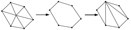
a) Vertex deletion method
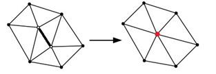
b) Side folding method
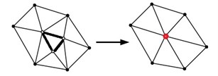
c) Triangular shrinkage method
In this paper, we introduced the weight value of the surface as an evaluation parameter. The larger the weight value was, the more curved the surface was, and the part should be kept; on the contrary, the smaller the weight value was, the flatter the surface was, and the part could be simplified, then the surface could be deleted. The weights, , were calculated as follows:
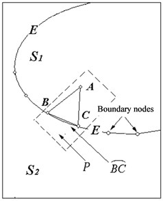
where is the normal vector of the triangle, is the normal vector of the three vertices of the triangle on the spline surface. is the angle between the vector and . The direction points to the outside of the model, 1, 2, 3, as shown in Fig. 5 and Fig.6.
Fig. 5The weight calculation diagram
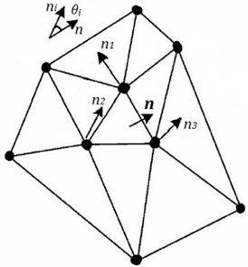
Fig. 6The surface boundary reconstruction principle
5. Residual entity reconfiguration
To verify the results of the algorithm, an example model was built using AutoCAD, as shown in Fig. 7. In the following, the simultaneous fitting of the spline surfaces in the model was performed based on the distance field of the spline surfaces. The example model was composed of eight surfaces, including a spline surface, a column surface and a plane surface. The size of the voxel of the distance field was an important parameter in the distance-field-based spline fitting process, and the definition of the size directly affected the number of facets to be fitted, the accuracy of the fit, and thus the error before and after the fit. Fig. 7 reflected the results generated by the distance field-based simultaneous fitting algorithm for the example model, where (a) the voxel size was set to 1.0 and (b) the fit was set to 4.0. From Fig. 8, the results of the model for fitting and remaining entity reconstruction are shown.
Fig. 7Results of patches in spline surface fitting
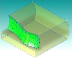
a)1
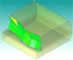
b)4
Fig. 8Results of fitting and the remaining solid reconstruction
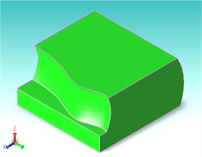
a) Original solid
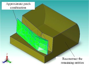
b) Reconstruction solid
As shown in Table 1, the sample surface fitting tests based on the distance field were performed on the example model using 0.5, 1.0, and 4.0, respectively. The test results were compared in terms of the number of facets obtained from the fitting, the area of the surface, and the area error before and after the fitting. The results in the table showed that the error between the area of the fitted surface combination and the area of the original sample surface was small after fitting the sample surface in the model, which proved that the algorithm was reasonable and reliable. Moreover, as the voxel size increased, the number of facets gradually decreased and the area error gradually increased. Therefore, 1.0 was a reasonable compromise between the number of voxels and the area error.
Table 1Spline fitting results of different voxel sizes in distance field
Model name | Number of patches | Area / (cm2) | Area error |
Original surface | 1 | 11336 | – |
Fitting curved surface (0.5) | 268 | 11302 | 0.00293 |
Fitting curved surface ( 1.0) | 164 | 11283 | 0.00461 |
Fitting curved surface (4.0) | 48 | 11264 | 0.00635 |
6. Conclusions
The algorithm of simultaneous fitting of adjacent spline surfaces based on distance fields was introduced. A set of planar slices was obtained by using the equivalence surface extraction method to achieve an accurate fitting of the spline surface. Simultaneously, the surface slices were simplified and the remaining entities were reconstructed, which not only effectively simulated the geometry of the spline surface, but also ensured the computational efficiency.
The method of simultaneous fitting of adjacent spline surfaces based on distance fields was proposed. An approximate representation of adjacent spline surfaces in CAD models using surfaces supported in the MC calculation program was implemented. This paper avoided the problem of overlap/gap that would arise from separate fitting processes by generating a distance field for the spline surfaces and then using the equivalent surfaces of the distance field to fit the adjacent spline surfaces simultaneously.
References
-
M. Sabin, “Two-sided patches suitable for inclusion in a B-spline surface,” in Proceedings of the international conference on Mathematical methods for curves and surfaces II Lillehammer, pp. 409–416, 1998.
-
S. A. Coons, “Surface patches and B-spline curves,” Computer Aided Geometric Design, pp. 1–16, 1974, https://doi.org/10.1016/b978-0-12-079050-0.50006-0
-
F. Yamaguchi, Curves and Surfaces in Computer Aided Geometric Design. Springer Science & Business Media, 1988.
-
Y. Zheng et al., “An improved NAMLab image segmentation algorithm based on the earth moving distance and the CIEDE2000 color difference formula,” in Intelligent Computing Theories and Application, Vol. 13393, pp. 535–548, 2022, https://doi.org/10.1007/978-3-031-13870-6_45
-
Z. Li, X. Zhou, and W. Liu, “A geometric reasoning approach to hierarchical representation for B-rep model retrieval,” Computer-Aided Design, Vol. 62, pp. 190–202, May 2015, https://doi.org/10.1016/j.cad.2014.05.008
-
G. M. Turner, I. S. Falconer, B. W. James, and D. R. Mckenzie, “Monte Carlo calculation of the thermalization of atoms sputtered from the cathode of a sputtering discharge,” Journal of Applied Physics, Vol. 65, No. 9, pp. 3671–3679, May 1989, https://doi.org/10.1063/1.342593
-
R. F. Aaronson, “A Monte Carlo model for quality assurance of intensity-modulated radiotherapy,” Ph.D. Thesis, p. 30890, 2003.
-
G. P. Skrebkov, A. S. Lozhkin, and S. N. Lozhkin, “Le Chatelier’s principle and its adaptation for closure of averaged equations of hydrodynamics,” Russian Meteorology and Hydrology, Vol. 32, No. 5, pp. 320–327, May 2007, https://doi.org/10.3103/s1068373907050056
-
E. Catmull, “A subdivision algorithm for computer display of curved surfaces.,” The University of Utah ProQuest Dissertations Publishing, 1974.
-
B. Braithwaite et al., “Optimized curve design for image analysis using localized geodesic distance transformations,” in IS&T/SPIE Electronic Imaging, Vol. 9399, pp. 9–19, Mar. 2015, https://doi.org/10.1117/12.2077826
-
G. Borgefors, “Distance transformations in digital images,” Computer Vision, Graphics, and Image Processing, Vol. 34, No. 3, pp. 344–371, Jun. 1986, https://doi.org/10.1016/s0734-189x(86)80047-0
-
Y. Zhao and J. Mao, “Equivalent Surface Impedance-Based Mixed Potential Integral Equation Accelerated by Optimized H – Matrix for 3-D Interconnects,” IEEE Transactions on Microwave Theory and Techniques, Vol. 66, No. 1, pp. 22–34, Jan. 2018, https://doi.org/10.1109/tmtt.2017.2731956
-
W. E. Lorensen and H. E. Cline, “Marching cubes: A high resolution 3D surface construction algorithm,” ACM SIGGRAPH Computer Graphics, Vol. 21, No. 4, pp. 163–169, Aug. 1987, https://doi.org/10.1145/37402.37422
-
C. Stucker and K. Schindler, “ResDepth: A deep residual prior for 3D reconstruction from high-resolution satellite images,” ISPRS Journal of Photogrammetry and Remote Sensing, Vol. 183, pp. 560–580, Jan. 2022, https://doi.org/10.1016/j.isprsjprs.2021.11.009
-
B. Li et al., “A coupled high-resolution hydrodynamic and cellular automata-based evacuation route planning model for pedestrians in flooding scenarios,” Natural Hazards, Vol. 110, No. 1, pp. 607–628, Jan. 2022, https://doi.org/10.1007/s11069-021-04960-x
About this article

The authors have not disclosed any funding.
The datasets generated during and/or analyzed during the current study are available from the corresponding author on reasonable request.
The authors declare that they have no conflict of interest.
