Damage detection of composite plate based on an improved DAS algorithm by time difference due to anisotropy

Liu, Li; Xia, Qingwei; Cao, Shuhao; Ma, Shiwei; Liu, Yanyan

doi:10.21595/jve.2020.21287

Journal of Vibroengineering

Browse Journal

Submit article

Published: 21 November 2020

Check for updates

Damage detection of composite plate based on an improved DAS algorithm by time difference due to anisotropy

Li Liu¹

Qingwei Xia²

Shuhao Cao³

Shiwei Ma⁴

Yanyan Liu⁵

^{1, 2, 3, 4, 5}School of Mechanical and Electrical Engineering and Automation, Shanghai University, Shanghai, China

Corresponding Author:

Yanyan Liu

Cite the article Download PDF

Downloads 1517

WoS Core Citations 2

CrossRef Citations 3

Abstract

This paper proposes a damage detection method based on an improved DAS imaging algorithm by introducing time difference due to anisotropy of composite material. First, the finite element characteristic frequency method is used to obtain the dispersion curve of the composite plate, and the validity of the dispersion curve is verified. Next, the average phase velocity of the Lamb wave at mixed modes in the composite plate is obtained by two-dimensional Fourier transform (2-D FFT). The mixed modal group velocity is calculated according to the corresponding phase velocity, the mean change rate of the phase velocity and the dispersion curve obtained by simulation. The time difference due to anisotropy of composite material is investigated, and the damage location is estimated by the delay-and-sum (DAS) imaging algorithm. Experiments on carbon fiber multilayer composite plates verify the effectiveness of the proposed method.

Damage detection of composite plate based on an improved DAS algorithm by time difference due to anisotropy

1. Introduction

Composite materials have many applications in aerospace, machinery and other industries due to the characteristics of light weight, high strength and long life [1]. In order to avoid property damage caused by safety accidents, material damage needs to be detected. Among the many detection methods, ultrasound imaging has been widely used due to its characteristics of non-destructive detection.

Due to its long propagation distance, low cost, and sensitivity to various damages, Lamb waves as a type of ultrasound are widely used in material damage detection [2]. Zhenqing Liu et al. [3] used two-dimensional Fourier transform to identify the mode of Lamb wave in aluminum plates. Wang et al. [4] proposed a delay-and-sum (DAS) algorithm to image damage in aluminum plates. Haiyan Zhang et al. [5] analyzed the propagation characteristics of Lamb waves in a layered anisotropic composite plate using the global matrix method. Rhee et al. [6] studied the group velocity of Lamb waves in composite plates. Sheen et al. [7] improved the RAPID algorithm to study lamb wave tomographic images. Linwen Zhang et al. [8] used the finite element characteristic frequency method to obtain the dispersion curve of the composite plates. Sikdar et al. [9] studied the effect of debonding damage on Lamb wave propagation in composites at variable temperatures.

Due to the characteristics of long Lamb wave propagation distance and sensitivity to damage, damage detection can be performed on plate-shaped composite materials. However, during propagation, Lamb waves have dispersion effects and multiple modes. In order to prevent modal aliasing, low frequency excitation signals or modal separation from the received signals are generally used for isotropic panels. However, because of the anisotropic characteristics of the layered composite plate and the variability of Lamb wave propagation between layers, the received signals from a multilayer composite plate are very complicated, thus it is difficult to perform modal separation. This brings challenges to signal analysis and damage identification.

This paper proposes a damage detection method based on an improved DAS algorithm without mode separation of Lamb waves. First, the finite element characteristic frequency method is used to obtain the dispersion curve of the composite plate, and the effectiveness of the dispersion curve of the single-layer composite plate is verified. Next, the average phase velocity of the Lamb wave in the mixed mode in the composite plate is obtained by two-dimensional Fourier transform. Based on the phase velocity and the simulated dispersion curve of the composite plate, the mean change rate of the mixed-mode phase velocity is calculated. Using the average mixed-mode phase velocity and the mean change rate of the mixed-mode phase velocity, the group velocity of the Lamb wave mixed mode is calculated. Due to the anisotropic characteristics of the composite plates, the time difference of different paths in the same direction is calculated based on the peaks of waveform. Damage location is estimated by improving the DAS algorithm with the effect of time difference. Experiments on carbon fiber multilayer composite plates are conducted to verify the effectiveness of this method.

2. Imaging principle

2.1. Finite element method for dispersion curve calculation

2.1.1. Fundamental

There is an essential relationship between the elastic wave and the vibration of the elastic body. The vibration of the elastic body is the simple resonance of the particles at different positions at their respective equilibrium positions. Vibration propagates through elastic media to form traveling waves to propagate energy. The wave equation in an elastic body is derived from the constitutive relationship and the equation of motion.

The wave equation of free propagation in an infinite anisotropic elastic material, its displacement is expressed as:

1

C_{i j k l} \frac{\partial^{2} u_{k}}{\partial x_{j} x_{i}} = ρ \frac{\partial^{2} u_{i}}{\partial t^{2}},

where $C_{i j k l}$ is the elastic matrix, $x_{i}$ is the coordinate system, $u_{i}$ is displacement ( $i$ , $j$ , $k$ , $l =$ 1, 2, 3).

The simple harmonic motion of the particles at their respective equilibrium positions is:

2

u = u_{m} e^{i ω t},

where $u_{m}$ is the vibration amplitude, $ω$ is the angular frequency.

From Eqs. (1) and (2), the intrinsic equations in anisotropic materials are:

3

(ρ ω^{2} δ_{i m} - C_{i k l m} k_{i} k_{l}) u_{m} = 0,

where $ρ$ is the material density; $δ_{i m}$ is the Kronecker delta; $k$ is the wave number; $i$ , $k$ , $l$ , $m$ is the tensor subscript.

Therefore, using the finite element simulation method to solve the problem of the free vibration equation of the structure can be simplified to solve the following characteristic equation:

4

K U - ω^{2} M U = 0,

where $ω$ is the characteristic frequency of the structure, $U$ is the displacement vector matrix of the vibration form corresponding to the characteristic frequency, $K$ is the stiffness matrix, $M$ is the mass matrix.

In order to analyze the propagation characteristics of ultrasonic waves in plate-like structures, consider the following free boundary conditions:

5

T_{i} = C_{i j k l} \frac{\partial u_{k}}{\partial x_{l}} n_{j} = 0,

where $n_{j}$ is the axial component of the normal vector $n$ outside the boundary unit.

According to Bloch-Floquet theorem, the solution of the wave equation has the following form:

6

u (r, t) = e^{i (k, r - ω t)} u_{k} (r),

where $k = {[k_{x}, k_{y}, k_{z}]}^{T}$ is Bloch wave vector. $u_{k} (r)$ is a function with a spatial period and can be calculated as:

7

u (r + L, t) = e^{i [k \cdot (r + l) - ω t]} u_{k} (r + L) = u (r, t) e^{i k l},

where $L$ is the lattice translation vector.

Due to the periodicity of the infinite plate structure and displacement, it is determined that the acoustic wave propagation characteristics in the plate can be studied by analyzing a period (a cell). Therefore, according to the periodic boundary conditions in the formula, the characteristic frequency corresponding to different Bloch wave vectors can be solved to obtain the dispersion relationship of the acoustic wave propagation in the plate.

2.1.2. Finite element characteristic frequency method

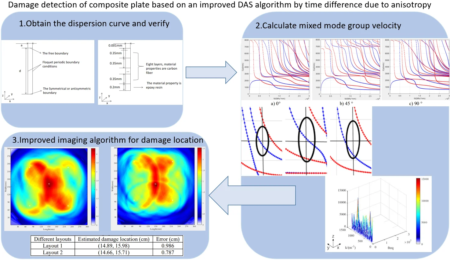
The paper uses COMSOL MULTIPHYSICS finite element simulation software, combined with the finite element characteristic frequency method, to calculate the dispersion curve of the Lamb wave in the anisotropic composite plate [8, 10]. Considering the infinite plate structure with a thickness of 2 $d$ in the $z$ direction, in order to facilitate the calculation of the dispersion curve in the board, only the simulation model shown in Fig. 1 was selected. Use Floquet periodic boundary conditions in the $x$ direction ( $a$ in the figure is the distance between the source boundary and the target boundary). For the non-wave vector $y$ -direction inner boundary of the plate, it also needs to be considered as a periodic boundary and be processed accordingly. The characteristic frequency is solved according to the eigenwave vector $k_{x}$ in the $x$ direction. Due to the symmetrical (antisymmetric) boundary conditions, the vibrations in the plate are symmetrical (antisymmetric) about the center plane in the $z$ direction, so that the finite element model is simplified to half of the original model. The symmetric and antisymmetric modes of the dispersion curve are obtained by setting symmetric and antisymmetric boundary conditions, respectively.

Fig. 1Dispersion curve by finite element method

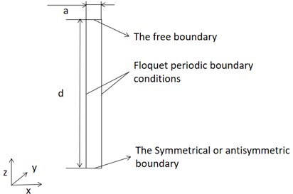
The finite element characteristic frequency solution method is used to calculate the dispersion curve of the single-layer carbon fiber composite board. The mechanical properties of 0° single-layer carbon fiber plate with the fiber direction in the $x$ direction are shown in Table 1. The carbon fiber density is 1800 kg/m³. $d$ takes 0.5 mm, a takes 0.001 mm. The elastic matrix of 45° and 90° fiber direction is obtained by transforming the values in Table 1. The dispersion curve obtained by the calculation is shown in Fig. 2.

Table 1Material mechanical properties of carbon fiber layer

E1 / GPa	E2 / GPa	E3 / GPa	G12 / GPa	G13 / GPa	G23 / GPa	$υ_{12}$	$υ_{13}$	$υ_{23}$
230	15	15	24	24	5.03	0.2	0.2	0.25

Fig. 2Dispersion curve of single layer carbon fiber plate

a) 0°

b) 45 °

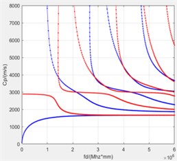
c) 90 °

In order to verify the effectiveness of the dispersion curve, the simulation model shown in Fig. 3(a) was constructed with a plate length of 100 mm. During the experiment, the position of the excitation sensor remains unchanged, and a set of data is measured at a distance of 5 mm from the receiving sensor. According to the dispersion curve obtained from the simulation, the frequency of the 0°-direction excitation signal is 1 MHz, the phase velocity of the A0 mode is 3000 m/s, and the group velocity is 3598 m/s. The frequency of the 45°-direction excitation signal is 2 MHz, the S0 mode phase velocity is 3230 m/s, and the group velocity is 2030m/s. The frequency of the 90°-direction excitation signal is 1MHz, the phase velocity of the S0 mode of 2810 m/s and the group velocity is 2520 m/s.

Fig. 3Experimental verification

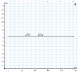
a) Simulation model

b) Receive signals

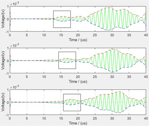
Take the envelope of the received signal in turn and find the peak time of the direct wave. The received signals with a propagation distance of 10 mm, 15 mm, and 20 mm in the 0° direction are shown in Fig. 3(b). The direct signal is inside the rectangular frame in the figure. The peak time of the direct wave obtained from the experiment is shown in Table 2.

Table 2Peak time of direct wave (μs)

	10 mm	15 mm	20 mm	25 mm	30 mm	35 mm	40 mm	45 mm	50 mm
0°	15.48	16.72	18	19.2	20.8	22.3	23.6	25	26.3
45°	15.04		18.7	21.46	24.22	26.8	29.52
90°		21.98	24.5	26.2	28.02	30.52	32	34.4	36.22

The signals received at some locations in the experiment cannot distinguish the direct wave, and the peak time of the direct wave cannot be determined. Fit the data in Table 2 to calculate the group velocity. The calculated group velocity and the error from the theoretical value are shown in Table 3.

Table 3Comparison between group velocity theory and experiment

Direction	Theoretical value (m/s)	Experimental value (m/s)	Error
0°	3598	3636.5	1.07 %
45°	2030	2020.8	0.45 %
90°	2520	2479.1	1.62 %

The experimental results show that the theoretical value and the actual value are consistent, verifying the effectiveness of the method.

2.1.3. Calculation of dispersion curve of the multilayer composite plate

The finite element characteristic frequency method is used to calculate the dispersion curve of the multilayer composite plate. The composite plate is composed of 17 layers, of which the upper eight layers and the lower eight layers are carbon fiber, and the middle layer is epoxy resin. The thickness of the carbon fiber layer is 0.35 mm, and the thickness of the epoxy resin layer is 0.4 mm. The carbon fiber layers are arranged in a cross pattern (0°/90°), that is, the carbon fiber direction of the previous layer differs from the carbon fiber direction of the next layer by 90°. The simulation model is shown in Fig. 4.

Fig. 4Multilayer composite plate simulation model

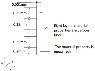
The material mechanical properties of carbon fiber layers are shown in Table 1. The Young’s modulus of the epoxy resin adhesive layer is 3.35 GPa, the density is 1150 kg/m³, and the Poisson’s ratio is 0.38. Take the fiber direction of the top layer of the multilayer composite plate as the 0° direction. The dispersion curve of the multilayer composite plate is shown in Fig. 5.

Fig. 5Dispersion curve of multilayer composite plate

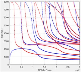
a) 0°

b) 45 °

c) 90 °

2.2. Basic principle of two-dimensional Fourier transform

The Fourier transform converts the signal in the time domain to the frequency domain, and the frequency domain signal is transformed into the wavenumber domain by spatial Fourier transform, as expressed by Eq. (8):

8

H (k, f) = \int_{- \infty}^{+ \infty} \int_{- \infty}^{+ \infty} u (x, t) e^{i (k x + ω t)} d x d t,

where $u (x, t)$ is the signal in the time domain, $ω = 2 π f$ is the angular frequency, $k$ is the wave number $k = ω / c$ , $c$ is the phase velocity.

The two-dimensional Fourier transform algorithm is able to measure the amplitude and velocity of different modes at the same frequency [3]. Thus, it is possible to determine the velocity of Lamb wave without mode separation by averaging among several adjacent modes at the same frequency.

2.3. Imaging method based on average group velocity and DAS algorithm

Amplitudes in frequency domain and spatial domain for one group of the received signals on a non-damaged plate are obtained by two-dimensional Fourier transform, which indicates the energy of the received signal at a superposition of several modes. The two-thirds of the maximum amplitude is taken as a reference. The phase velocities in each group where the energy amplitudes are greater than the reference value are averaged to obtain a phase velocity for the mixed modes. The overall average phase velocity $c_{p}$ is averaged among multiple groups.

According to the frequency thickness product in dispersion curve, the change rates of several modes near $c_{p}$ at a certain frequency thickness product are obtained. The average group velocity $c_{g}$ is calculated as follows:

9

c_{g} = \frac{{c_{p}}^{2}}{c_{p} - \bar{Δ c_{p}}},

where $c_{p}$ is the average phase velocity, and $\bar{∆ c_{p}}$ is the average transformation rate of phase velocity at a certain frequency thickness product. An $\bar{∆ c_{p}}$ be calculated by Eq. (10):

10

\bar{Δ c_{p}} = \frac{\sum_{i = 1}^{n} (f_{d}) \frac{d c_{p i}}{d (f_{d})}}{n},

where $f_{d}$ is the frequency-thickness product, and $n$ is the number of modes selected near the average phase velocity.

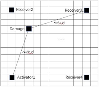
The damage detection is performed using the delay-and-sum algorithm [4], as shown in Fig. 6. The scattered signal is obtained by subtracting the baseline signal from the signal in the damaged plate. As the wave speeds at different positions along the same direction of anisotropic composite plate are different, a non-damaged plate is used as a calibration. The time difference between signals of non-damaged plate is used as a time delay in the imaging method. The pixel value $A (x, y)$ of each pixel in the pixel map is as follows:

11

A (x, y) = \sum_{n = 1}^{N} f_{n x y} (t + t_{n}),

where $t_{n}$ is the time difference of the $n$ th path, $N$ is the number of paths, $f_{n} (t)$ is the envelope of the scattered signal for each path, and $t$ is the propagation time of the scattered signal.

$t$ can be calculated as:

12

t = \frac{r_{a n} (x, y) + r_{s n} (x, y)}{c_{g}},

where $r_{a n} (x, y)$ and $r_{s n} (x, y)$ represent the distances from the grid $(x, y)$ to the excitation sensor and the receiving sensor, respectively.

Fig. 6DAS imaging method

3. Experiment and results

3.1. Experimental setup

Experiments were performed on two multilayer T700 carbon fiber composite plates of the same size as shown in Fig. 7(a) and Fig. 7(b). The two composite plates are both 300 mm long, 300 mm wide and 6mm high, and the layers arrangement of the two plates are the same as described in Section 2.1. One plate is non-damaged, and for the other plate a PZT piezoelectric sheet of 14 mm diameter is isolated and debonded at the center position (15, 15) cm of the epoxy resin layer to represent a damage.

The experiment setup for damage localization in composite plate is shown in Fig. 7(c). An arbitrary signal generator 33250A produced by Agilent is used to excite Lamb wave signals. A 4-channel mixed signal oscilloscope DPO5034B produced by Tektronix is used to receive signals from the plate. All the PZT sensors used in the experiment are identical with a center frequency of 200 kHz.

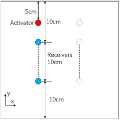
Signals from 21 transmitter-receiver pairs are collected for the calculation of average phase velocity by the 2-D FFT as shown in Fig. 8, where the red circle represents the excitation sensor which is fixed, and the blue circle is the reception sensor which moves along $x$ -direction and $y$ -direction, respectively.

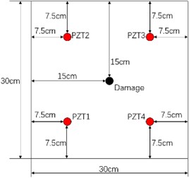
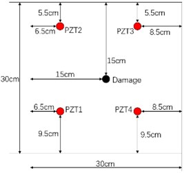
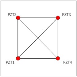
Two layouts of the sensors as shown in Figs. 9(a) and (b) are used to determine the damage position for the same damage. Fig. 9(c) shows the 6 sensing paths of each layout. Positions of sensors in layout 1 are: PZT1 (7.5, 7.5) cm, PZT2 (7.5, 22.5) cm, PZT3 (22.5, 22.5) cm, PZT4 (22.5, 7.5) cm. Positions of sensors in layout 2 are: PZT1 (6.5, 9.5) cm, PZT2 (6.5, 24.5) cm, PZT3 (21.5, 24.5) cm, PZT4 (21.5, 9.5) cm. The detection area is divided into 800 × 800 = 640000 grids, and the area of each grid is 0.375 × 0.375 mm².

Fig. 7Experimental setup diagram

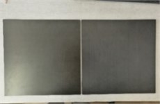
a) Two composite plates

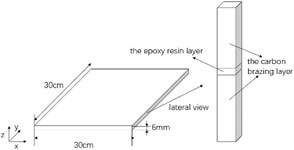
b) Plate size

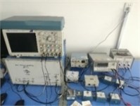
c) Laboratory equipment

Fig. 8Sensor layout for calculation of group velocity

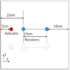
a) Along $x$ -axis direction

b) Along $y$ -axis direction

Fig. 9Sensor layout for damage localization

a) Sensor layout 1

b) Sensor layout 2

c) Sensing paths layout

3.2. Experimental results

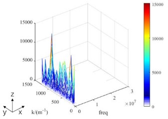
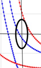
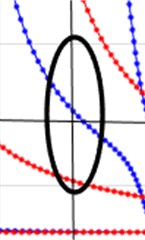
The two-dimensional Fourier transform of one group of signal is shown in Fig. 10(a). The phase velocity is calculated as 3585.6 m/s by averaging the nine sets of data. The frequency thickness product is 1.2 MHz∙mm. As shown in Fig. 10(b-d), from the dispersion curve, there are four modes whose velocities are near the average phase velocity (inside the black circle). The mode in 0° direction is A3. The modes in 45° direction are A2 and S2. The mode in 90° direction is A2. The mean change rate $\bar{∆ c_{p}}$ of the four modes is calculated as -3104.3. From Eq. (9), the corresponding group velocity is 1921.74 m/s.

Fig. 10Calculation of group velocity

a) 2-D FFT for phase velocity

b) 0°

c) 45°

d) 90°

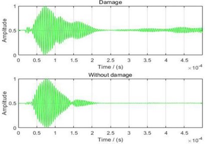
For damage localization, the excitation waveform is a 5-period sine wave modulated by a Hamming window, and the received signal from the non-damaged plate is used as a baseline signal. Fig. 11(a) shows received signals from the damaged plate and the non-damaged plate, respectively. The scattered signal is the subtraction between the above two received signals. Due to the anisotropy of the composite plate, the speeds in same directions are not exactly the same. From Fig. 9(c), it is seen that the directions of paths 1-2 and 3-4 in the non-damaged plate are the same, but the travel times at the peak amplitude of the two paths are different as shown in Fig. 11(b), which lead to a time difference $t$ . There are six paths in each sensor layout in Fig. 9(c), and paths in the same direction are considered as a pair. Among them, since the two diagonal lines make a 45° angle with the fiber direction, they can be regarded as a pair. The average time difference of the three pairs of paths is obtained. The time difference for sensor layout 1 is 22.22 μs, and the time difference for sensor layout 2 is 8.97 μs.

Fig. 11Waveforms of received signals and calculation of time difference

a) Waveforms from damaged and non-damaged plates

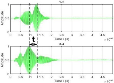
b) Time difference of two paths in same direction

Damage position estimation by our imaging method for both the sensor layouts are shown in Fig. 12, where the black circles represent the actual damage locations and the white circles represent the damage locations estimated by our method.

The errors between the estimated damage position and the actual damage position (15, 15) cm are given in Table 4. The errors may be caused by the inaccuracy calculation of the group velocity of the mixed modes and the disturbance of the received signals.

Table 4Damage positioning error

Different layouts	Estimated damage location (cm)	Error (cm)
Layout 1	(14.89, 15.98)	0.986
Layout 2	(14.66, 15.71)	0.787

Fig. 12Imaging results

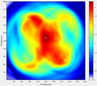
a) Imaging for Layout 1

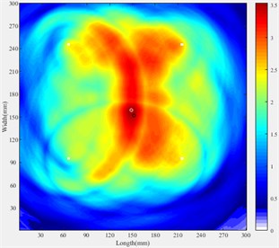
b) Imaging for Layout 2

4. Conclusions

This paper presents a method for damage localization on composite plate by an improved DAS algorithm using Lamb waves without mode speration. Phase velocity of Lamb waves in composite plates was determined by using two-dimensional Fourier transform. The dispersion curve is obtained from the finite element characteristic frequency method. The group velocity is calculated from several mixed modes in the dispersion curve. Damage position is estimated by the delay-and-sum imaging method with introducing an anisotropic time difference. The experimental results show that the method is effective for the localization of damage. A better imaging may be achieved by more sets of 2D Fourier transform signals and more accurate time difference calculation methods.

References

Songping Liu, Engming Guo Present situation and prospects of nondestructive testing and evaluation technology for composites. Aeronautical Manufacturing Technology, Vol. 3, 2001, p. 30-32.

Search CrossRef
Alleyne D. N., Cawley P. The interaction of Lamb waves with defects. IEEE Transactions on Ultrasionc Ferroelectrics and Frequency Control, Vol. 39, Issue 3, 1992, p. 381.

Publisher
Zhenqing Liu, Dean Ta Mode identify of Lamb wave by means of 2-D FFT. Technical Acoustics, Vol. 4, 2000, p. 212-214+219.

Search CrossRef
Wang C. H., Rose J. T., Chang F. K. A synthetic time-reversal imaging method for structural health monitoring. Smart Materials and Structures, Vol. 13, Issue 2, 2004, p. 415-423.

Publisher
Haiyan Zhang, Zhengqing Liu, Donghui Lu Global matrix and its application to study on lamb wave propagation in layered anisotropic composite plates. Acta Materiae Compositae Sinica, Vol. 21, Issue 2, 2004, p. 111-116.

Search CrossRef
Rhee S. H., Lee J. K., Lee J. J. The group velocity variation of Lamb wave in fiber reinforced composite plate. Ultrasonics, Vol. 47, Issues 1-4, 2007, p. 55-63.

Publisher
Sheen B., Cho Y. A study on quantitative lamb wave tomogram via modified RAPID algorithm with shape factor optimization. International Journal of Precision Engineering and Manufacturing, Vol. 13, Issue 5, 2012, p. 671-677.

Publisher
Linwen Zhang, Shiwei Ma, Qian Cheng Lamb wave characteristic anysissis of anisotropic multierayer composite using finite ellent intrinsic frequency method. Nondestructive Testing, Vol. 4, 2017, p. 67-71.

Search CrossRef
Sikdar S., Fiborek P., Kudela P., et al. Effects of debonding on Lamb wave propagation in a bonded composite structure under variable temperature conditions. Smart Materials and Structures, Vol. 28, Issue 1, 2019, p. 015021.

Publisher
Liang Chen, Enbao Wang, Hao Ma Calculation of ultrasonic lamb wave dispersion curve of the thin plate by the finite element method. Research and Exploration in Laboratory, Vol. 11, 2014, p. 28-31.

Search CrossRef

Cited by

Damage imaging method for composites laminates based on sparse reconstruction of single-mode Lamb wave

Hui Wu | Shiwei Ma | Bingxu Du

(2022)

Methods and Applications for Modeling and Simulation of Complex Systems

Hui Wu | Shiwei Ma | Bingxu Du

(2022)

Lamb Wave-Based Damage Localization and Quantification in Composites Using Probabilistic Imaging Algorithm and Statistical Method

Jiahui Guo | Xianping Zeng | Qijian Liu | Xinlin Qing

(2022)

About this article

Received

08 January 2020

Accepted

23 June 2020

Published

21 November 2020

SUBJECTS

Fault diagnosis based on vibration signal analysis

DOI

https://doi.org/10.21595/jve.2020.21287

Keywords

composite plate; mixed mode; two-dimensional Fourier transform; damage detection

Acknowledgements

This work was supported by the National Natural Science Foundation of China with Grant Nos. 61671285.

This is an open access article distributed under the Creative Commons Attribution License, which permits unrestricted use, distribution, and reproduction in any medium, provided the original work is properly cited.

Previous article in issue Previous Next article in issue Next

Research article

2022 02 05

Composite plate damage localization based on modal parameters

Jiayu Cao, Hongliang Yu, Jin Yan, Jianbin Liao

Research article

2017 10 21

Detection and localization of closely distributed damages via lamb wave sparse reconstruction

Jiadong Hua, Chen Lu, Zili Wang, Jing Lin

Research article

2017 08 15

Study of modal acoustic emission to monitor the impact damage in a composite plate

Baochun Xu, Jingqiu Wu, Mulan Wang

Research article

2015 09 18

A new damage imaging method based on lamb wave wavenumber response and PZT 2D cross-shaped array

Lei Qiu, Shenfang Yuan, Zhongqing Su, Bin Liu

L. Liu, Q. Xia, S. Cao, S. Ma, and Y. Liu, “Damage detection of composite plate based on an improved DAS algorithm by time difference due to anisotropy,” Journal of Vibroengineering, Vol. 22, No. 8, pp. 1747–1757, Nov. 2020, https://doi.org/10.21595/jve.2020.21287

Copy Extrica

Copied to clipboard!

TY  - JOUR
DO  - 10.21595/jve.2020.21287
UR  - https://doi.org/10.21595/jve.2020.21287
TI  - Damage detection of composite plate based on an improved DAS algorithm by time difference due to anisotropy
T2  - Journal of Vibroengineering
AU  - Liu, Yanyan
AU  - Liu, Li
AU  - Xia, Qingwei
AU  - Cao, Shuhao
AU  - Ma, Shiwei
PY  - 2020
DA  - 2020/11/21
PB  - JVE International Ltd.
SP  - 1747-1757
IS  - 8
VL  - 22
SN  - 1392-8716
SN  - 2538-8460
ER  - 

Copy Ris

Copied to clipboard!

@article{Liu_2020,
	doi = {10.21595/jve.2020.21287},
	url = {https://doi.org/10.21595/jve.2020.21287},
	year = 2020,
	month = {nov},
	publisher = {{JVE} International Ltd.},
	volume = {22},
	number = {8},
	pages = {1747--1757},
	author = {Yanyan Liu and Li Liu and Qingwei Xia and Shuhao Cao and Shiwei Ma},
	title = {Damage detection of composite plate based on an improved {DAS} algorithm by time difference due to anisotropy},
	journal = {Journal of Vibroengineering}
}

Copy Bibtex

Copied to clipboard!

[1]Y. Liu, L. Liu, Q. Xia, S. Cao, and S. Ma, “Damage detection of composite plate based on an improved DAS algorithm by time difference due to anisotropy,” Journal of Vibroengineering, vol. 22, no. 8, pp. 1747–1757, Nov. 2020, doi: 10.21595/jve.2020.21287.

Copy IEEE

Copied to clipboard!

Liu, Yanyan, Li Liu, Qingwei Xia, Shuhao Cao, and Shiwei Ma. “Damage Detection of Composite Plate Based on an Improved DAS Algorithm by Time Difference Due to Anisotropy.” Journal of Vibroengineering 22, no. 8 (November 21, 2020): 1747–57. https://doi.org/10.21595/jve.2020.21287.

Copy Chicago

Copied to clipboard!

Damage detection of composite plate based on an improved DAS algorithm by time difference due to anisotropy

Abstract

1. Introduction

2. Imaging principle

2.1. Finite element method for dispersion curve calculation

2.1.1. Fundamental

2.1.2. Finite element characteristic frequency method

2.1.3. Calculation of dispersion curve of the multilayer composite plate

2.2. Basic principle of two-dimensional Fourier transform

2.3. Imaging method based on average group velocity and DAS algorithm

3. Experiment and results

3.1. Experimental setup

3.2. Experimental results

4. Conclusions

References

Cited by

About this article

Related Articles