On a three-dimensional neural network model

1. Introduction

The theory of neural networks appeared as an attempt to understand the structure and principles of the functioning of the human brain. Now it is rich in results and practically significant field of research in natural sciences. Artificial neural networks (ANN) can be understood as computing systems inspired by biological neural networks. Their mathematical models can be formulated in terms of systems of quasi-linear differential equations of the form Eq. (1). Each dependent variable $x_i$ is associated with a neuron. It accepts signals from other neurons (this is called input) and elaborates its own signal (it is called output) which is sent to a network. The nonlinearity is called the response function, or activation function. Usually, a sigmoidal function like $f\left(z\right)=1/(1+\mathrm{e}\mathrm{x}\mathrm{p}(-z\left)\right)$ or $\mathrm{t}\mathrm{a}\mathrm{n}\mathrm{h}\left(z\right)$ is used. Recent attempts to introduce other response functions may be found in [6]-[9]. The system:

Appears in neurodynamics [1], [2]. It is of general nature, and for appropriate choice of parameters $a_i$ and $b_j$ it may have rich dynamics. Moreover, for sufficiently large $n$ it can approximate (on a finite interval) any dynamical system [3]. The dynamics of solutions is a valuable object of investigation. Especially future states of a modeled neural networks are important to know. For this, the analysis of the phase space is needed. Future states are heavily dependent on attractors of the system, [4], [5]. In this note we will show that the three-dimensional system of the form Eq. (1) can have stable equilibria in the form of stable focuses. For the appropriate choice of parameters, it can have limit cycles attracting other solutions.

2. Two-dimensional system

Consider the system:

Proposition 1. System Eq. (2) can have stable critical points of the type stable focus.

Proof by construction the example. Set $a_{11}=k$, $a_{12}=$ 1.5, $a_{21}=$ –1.5, $a_{22}=k$, $k=$ 0.2, $b_1=b_2=$1, see Fig. 1.

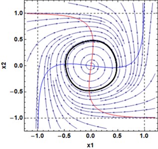
Proposition 2. System Eq. (2) can have a limit cycle.

Proof by constructing the example. Set $a_{11}=k$, $a_{12}=$ 1.5, $a_{21}=$ –1.5, $a_{22}=k$, $k=$ 1.2, $b_1=b_2=$1, see Fig. 2.

Fig. 1Stable focus as in Proposition 1

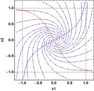
Fig. 2Limit cycle as in Proposition 2

3. Three-dimensional system

Consider the three-dimensional system of the form Eq. (1):

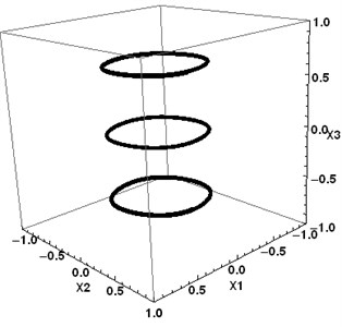
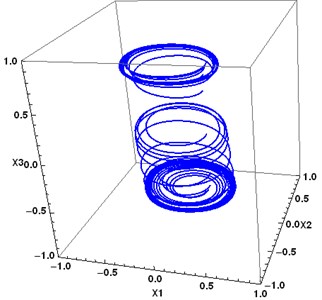
Proposition 3. System Eq. (3) can have three limit cycles.

Proof by construction the example. Let the coefficient matrix in Eq. (3) be:

and see Fig. 4.

The nullclines for the system Eq. (3) are given by the relations:

There are three periodic solutions. The respective trajectories are located in three planes (blue ones in Fig. 3). The critical points inside the limit cycles have the following characteristic numbers: ${\lambda }_1=$ –0.32, ${\lambda }_{\mathrm{2,3}}=$ 0.2±1.5i for the critical points at (0; 0; ±0.65857). The central critical point (0;0;0) has ${\lambda }_1=$ 0.2, ${\lambda }_{\mathrm{2,3}}=$0.2 ±1.5i. Trajectories go away from the central critical point.

Fig. 3Nullclines of the system Eq. (3), matrix A

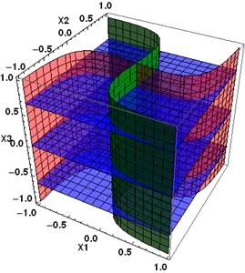
Fig. 4Three periodic trajectories of the system Eq. (3)

4. Perturbation of three-dimensional system

Let the coefficients of the system Eq. (3) be perturbed as:

Fig. 5Nullclines of the system Eq. (3) with the coefficient matrix A1

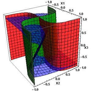
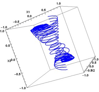
Fig. 6Two periodic attractors of the system Eq. (3), coefficient matrix A1, and converging some other trajectories. The middle limit cycles are destroyed

There are still three critical points at (–0.051; –0.039;0.68723), (0; 0; 0), (0.051; 0.039; –0.68723). Their characteristic numbers are: ${\lambda }_1=$ –0.3543, ${\lambda }_{\mathrm{2,3}}=$ 0$.$19±1.4946i for the first and the third critical points, and ${\lambda }_1=$0.2266, ${\lambda }_{\mathrm{2,3}}=$0.1866±1.5i for the central point.

Let the coefficients of the system Eq. (3) be perturbed as:

There are still three critical points at (0.0527; 0.6533; –0.76188), (0;0;0), (–0.0527; –0.6533; 0.76188). Their characteristic numbers are: ${\lambda }_1=$ –0.4434, ${\lambda }_{\mathrm{2,3}}=$ 0.089±1.1882i for the first and the third critical points, and ${\lambda }_1=$ 0.2921, ${\lambda }_{\mathrm{2,3}}=$ 0.1539±1.6632™ for the central point.

Fig. 7Nullclines of the system Eq. (3) with the coefficient matrix A2

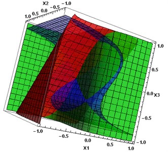
Fig. 8Two periodic attractors of the system Eq. (3), coefficient matrix A2, and converging trajectories

5. Conclusions

Dynamical systems, arising in neurodynamic, can have periodic attractors in the form of the limit cycles. Periodic attractors in two-dimensional systems appear as the result of Andronov-Hopf bifurcation, where the bifurcating parameter is the value at the main diagonal of the coefficients matrix $A$. Three-dimensional systems can have two attractors in the form of limit cycles. Small perturbation of the coefficient matrix $A$ can destroy limit cycles lying in a non-stable manifold (that is, in the middle plane in the example above). It seems that two side attractors (which were in stable manifolds) are preserved under the perturbations saving the types of the corresponding critical points. For practical purposes, special attention should be paid to perturbations that preserve the structure of the nullclines and, as a consequence, characteristics of equilibria (critical points).

References

-
S. Haykin, Neural Networks. A Comprehensive Foundation. Prentice Hall, 1998.
J. C. Sprott, Elegant Chaos. Singapore: World Scientic, 2010.
K.-I. Funahashi and Y. Nakamura, “Approximation of dynamical systems by continuous time recurrent neural networks,” Neural Networks, Vol. 6, No. 6, pp. 801–806, Jan. 1993, https://doi.org/10.1016/s0893-6080(05)80125-x
D. Ogorelova, F. Sadyrbaev, and V. Sengileyev, “Control in inhibitory genetic regulatory network models,” Contemporary Mathematics, Vol. 1, Oct. 2020, https://doi.org/10.37256/cm.152020538
I. Samuilik and F. Sadyrbaev, “Modelling three dimensional gene regulatory networks,” WSEAS Transactions on Systems and Control, Vol. 16, pp. 755–763, 2021.
A. Afzal, J. K. Bhutto, A. Alrobaian, A. Razak Kaladgi, and S. A. Khan, “Modelling and computational experiment to obtain optimized neural network for battery thermal management data,” Energies, Vol. 14, No. 21, p. 7370, Nov. 2021, https://doi.org/10.3390/en14217370
S.-L. Shen, N. Zhang, A. Zhou, and Z.-Y. Yin, “Enhancement of neural networks with an alternative activation function tanhLU,” Expert Systems with Applications, Vol. 199, p. 117181, Aug. 2022, https://doi.org/10.1016/j.eswa.2022.117181
E. Trentin, “Networks with trainable amplitude of activation functions,” Neural Networks, Vol. 14, No. 4-5, pp. 471–493, May 2001, https://doi.org/10.1016/s0893-6080(01)00028-4
H. Zhu, H. Zeng, J. Liu, and X. Zhang, “Logish: A new nonlinear nonmonotonic activation function for convolutional neural network,” Neurocomputing, Vol. 458, pp. 490–499, Oct. 2021, https://doi.org/10.1016/j.neucom.2021.06.067
About this article
ESF Project No. 8.2.2.0/20/I/003 “Strengthening of Professional Competence of Daugavpils University Academic Personnel of Strategic Specialization Branches 3rd Call”.
The datasets generated during and/or analyzed during the current study are available from the corresponding author on reasonable request.
The authors declare that they have no conflict of interest.