On attractors in systems of ordinary differential equations arising in models of genetic networks

1. Introduction

We study systems of ordinary differential equations, arising in applications. The following system:

first appeared in the study of neuronal networks [1]. It was applied later by several authors to treat genetic regulatory networks [2], [3] and telecommunication networks [4]. In this note, we focus on genetic networks. System Eq. (1) models the evolution of a genetic regulatory network (GRN). The interrelation between elements of a network is described by the regulatory matrix $W=\left(w_{ij}\right)$. A variable $x_i\left(t\right)$ stands for the expression of protein by an $i$-th gene. The main question is the future state of a network. The current state is described by the vector $X\left(t\right)=\left(x_1\left(t\right),\dots ,x_n\left(t\right)\right)$. Future states are represented by trajectories $X\left(t\right)$. The system has attracting sets in a phase space, which heavily influence the behavior of trajectories and other important properties of a network. The system Eq. (1) has at least one critical point (equilibrium) since nullclines intersect in the invariant parallelepiped $Q_n=\left\{0<x_i<1/v_i,i=1,\dots ,n\right\}$. The vector field, defined by system Eq. (1), is directed inward on the border of $Q_n$. Therefore, an attractor for trajectories of the system Eq. (1) must exist. Stable equilibria can appear in the system Eq. (1), but their number is finite. Stable equilibria are simple attractors. There are systems with a critical point, which is not attractive [5]. A stable periodic solution appears instead. Limit cycles can emerge from stable focuses as a result of Andronov – Hopf bifurcation. Attractors were constructed in systems with dimensions higher than three [6], [7]. These attractors are not solutions themselves, but they attract periodic solutions of a system. System (1) can exhibit chaotic behavior, which is not easy to detect. We would like to recall the example, which was obtained first in [8], then modified and analyzed in [9], [10]. In what follows, we recall this example and consider another one. Both examples are to be compared and supplied with related images.

2. Three-dimensional systems. First example

Consider system Eq. (1) for $n=$3 (three-dimensional system), $x_1\left(t\right)=x\left(t\right)$, $x_2\left(t\right)=y\left(t\right)$, $x_3\left(t\right)=z\left(t\right)$. We use the simplified notation $\left(x,y,z\right)$ now, to avoid indices:

Recall the modification [9] of the example, first obtained in [8]. Let the parameters be: $v_1=0.65$, $v_2=0.42$, $v_3=0.1$; ${\mu }_1=7$, ${\mu }_2=7$, ${\mu }_3=13;$${\theta }_1=0.5$, ${\theta }_2=$0.3, ${\theta }_3=$0.7. The coefficients $w_{ij}$ are elements of the regulatory matrix:

The nullclines of a system Eq. (2) are depicted in Fig. 1 together with some trajectories, tending to an attractor. The mutual disposition of nullclines and an attractor can be checked visually. The irregular behavior of solutions is shown in Fig. 2.

Fig. 1The nullclines of the system Eq. (2). The trajectory tending to an attractor (blue)

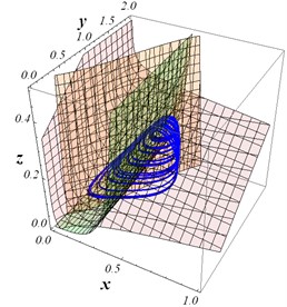
Fig. 2Solutions of system Eq. (2), with the initial conditions x1=0.9; y1=0.7; z1=0.11

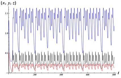
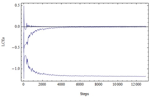
Fig. 3LE1= 0.011; LE2 = –0.008; LE3 = –1.173

There is one critical points: (0.3768; 1.5870; 0.2212). Linearization around this point yields the characteristic numbers $\lambda$: ${\lambda }_1=-1.2709$; ${\lambda }_{\mathrm{2,3}}=0.0504\pm 0.7378i$.

Lyapunov exponents of the system Eq. (2) (calculations made by the program lce.m by M. Sandri [11]).

The sum of two first Lyapunov numbers is positive. This is the evidence of chaotic behavior of solutions.

3. Three-dimensional systems. Second example

Consider system Eq. (1) for $n=$3 (three-dimensional system), $x_1\left(t\right)=x\left(t\right)$, $x_2\left(t\right)=y\left(t\right)$, $x_3\left(t\right)=z\left(t\right)$:

with the following parameters: $v_1=1$, $v_2=1$, $v_3=0.32$; ${\mu }_1=2.38$, ${\mu }_2=5.095$, ${\mu }_3=1.66$; ${\theta }_1=1.574$, ${\theta }_2=0.5362$, ${\theta }_3=1.5255$. The coefficients $w_{ij}$ are elements of the regulatory matrix:

The nullclines of the system Eq. (4) are depicted in Fig. 4 together with a trajectory. There are three critical points at (0.1126; 0.1260; 0.7926); (0.9709; 0.0010; 2.9674); (0.1862; 0.2274; 0.6596). Linearization around these points provides us with the characteristic numbers $\lambda$.

Fig. 4The nullclines of the system Eq. (4). The trajectory of system Eq. (4) forming the attractor.

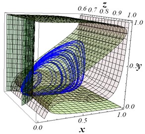
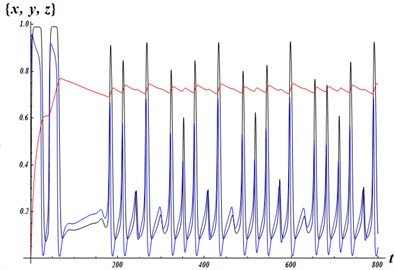
Fig. 5Solutions of system Eq. (4), with the initial conditions x0=0.1; y0=0.7; z0=0

The first and the third points possess characteristics of opposite nature. Both are saddle-focus points, the first point having stable focus, while repelling in the third dimension. The third point has unstable focus, but it is attractive in the remaining dimension. The second point is relatively far away of these two ones.

Three components of a solution with the initial conditions $x\left(0\right)=0.1$; $y\left(0\right)=0.7$; $z\left(0\right)=0$ are depicted in Fig. 5.

The dynamics of Lyapunov exponents is shown in Fig. 6.

The sum of the two first Lyapunov numbers is positive, and this is an indication of the chaotic behavior of solutions.

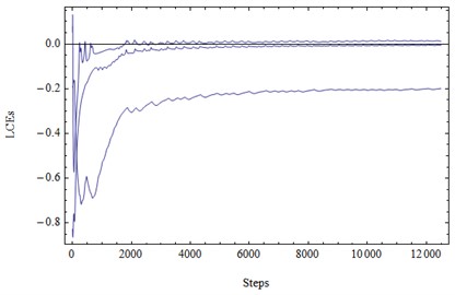
Fig. 6. LE₁= 0.014; LE₂= –0.004; LE₃= –0.197

4. Conclusions

In addition to the previously known attractor in a system of the form Eq. (2), another example of an attractor with chaotic behavior of solutions is obtained. The mechanisms of the appearance of the attractor in both examples are different. In the first example, the attractor exists in a vicinity of a single critical point, with an unstable two-dimensional manifold and a stable one-dimensional one.

The motion of trajectories in the second example: a trajectory enters the area of the equilibrium point ((0.1126; 0.1260; 0.7926), unstable in a one-dimensional manifold and stable in a two-dimensional manifold), trajectories leave this point and approach the critical point ((0.1862; 0.2274; 0.6596) stable in a one-dimensional manifold, unstable in a two-dimensional manifold). The movement of trajectories continues around the same point (0.1862; 0.2274; 0.6596).

To the best of the author’s knowledge, these are the only three-dimensional examples of chaotic behavior of solutions in systems of the form Eq. (1).