Abstract
In the paper, two new methods are developed and examined to implement a transfer function based approach in solving differential equations with Non-Zero initial conditions. A significant amount of time and effort is needed for solving differential equations theoretically or manually. Also, the obtained mathematical solutions to equations that represent various dynamic systems provide no graphical picture of the result. Using Simulink/MATLAB for modeling differential equations make the task of analyzing the behavior of systems easy and quick for the user. Beside, symbolic solutions and visual plots/graphs of the simulated results can be easily obtained and analyzed. Simulink uses different approaches to model a dynamic system such as differential equations in time domain (integrators based) or transfer function based and state space based. The paper addresses and compares different approaches used in Simulink for implementing block diagram based mathematical models of differential equations with non-zero initial conditions. Customarily, a transfer function based approach is used for analyzing systems with zero initial conditions. The paper demonstrated how to use a transfer function based approach for solving differential equations with non-zero initial conditions and two ways are devised to successfully implement the approach. To conclude, dynamic behavior of circuit and systems is analyzed and examined by obtaining graphical solutions with different approaches for chosen system parameters.
1. Introduction
Simulink (Simulation and Link) is a software package integrated within MATLAB which has becomes most used engineering software package in last few years among academics and industries. It provides a graphical user interface (GUI) environment where the user can draw the models in a way they could be drawn with a pencil and paper so that dynamic systems can be designed, tested, simulated and their behavior can be analyzed graphically. Building a block diagram based model in Simulink is simple and can be achieved with click-and-drag mouse operations. Simulink has a wide-ranging library of blocks and toolboxes for supporting both linear and nonlinear analysis. The constructed models are ordered so that both top-down and bottom-up approaches can be used. As Simulink works with MATLAB, it is easy to switch back and forth during the analysis process and take advantage of features offered in both the environments.
Simulink can solve models for both continuous and discrete-time (sampled time) components/systems or a hybrid of the two graphically and simulate many of the operational problems occur in the real world [1-3]. Most of the dynamic systems contain energy storage elements e.g., masses and springs in mechanical systems or inductors and capacitors in an electrical circuit and due to principle of conservation of energy these systems do not experience instantaneous changes in the state variables. Therefore, transients occur in the systems’ response before steady-state response values. Simulink is very visual and intuitive, and therefore has become a powerful tool for modeling and simulation of dynamic systems. Any system can be built easily in block diagram representation using Simulink and the simulation results are displayed quickly. Simulation algorithms and parameters can be changed in the middle of a simulation with natural results. MATLAB is undoubtedly an all-rounder tool for simulations, programming, graphs, measurement & automation and statistics for an engineer.
The Simulink tool is employed for numerical solving of differential equations describing systems e.g. in solving continuous systems that include a pendulum with an external source of force, wind created by the force of a ventilator, etc. There are many applications in electrical, mechanical, aerospace, robotics and civil engineering technology that require solving higher-order differential equations in a quick manner [4]. Differential equations of different orders play a pivotal role in diverse fields like mathematics, physics, electrical, mechanical and civil engineering and biological population modeling [5], etc. For modeling and analyzing systems in diverse engineering and scientific applications, Simulink uses different approaches such as differential equations (integrators based) or transfer function based or state space based [2, 6-9]. There is no need to model and transform differential equations (or difference equations) in a coded language or written program. The simulation analysis provides information about various performance parameters of the system, such as stability of the system, its step or impulse response, and its frequency response.
Simulink (a graphical editor tool) has an extensive set of blocks which can be used to realize various functions useful for simulation and analysis of dynamic systems. The blocks are grouped into various sub-libraries categorized using all-purpose functions e.g., Math Library (containing mathematical function blocks such as summer, gain, trigonometric, product, etc.), Sources library (containing common input functions such as sine, constant, ramp, clock, etc.), Continuous library (containing integrators), Sinks library (containing Scope, Display, To workspace blocks, etc.). Each Simulink blocks have a set of configurable parameters. Different properties and parameter values of the blocks arranged according to their functions can be modified in the related dialog boxes. The addition block can be configured to add or subtract two signals. Double-click on the block to change the signs.
Physical systems’ performance can be determined by employing related physical laws or equations that generally govern the systems. Physical systems can be represented mathematically as a set of differential equations or by using transfer function approach. Representing complex systems or systems having multiple inputs and outputs with differential equations or transfer functions is cumbersome. To avoid this, state space method is employed.
2. Theory
2.1. Solving differential equations with non-zero initial conditions
A differential equation is a mathematical equation for an unknown function of one or several variables that relates the value of the function itself and its derivatives of various orders. Ordinary differential equations (ODE) are derivatives of a dependent variable with respect to one independent variable, usually time. Ordinary differential equations (ODE) play a fundamental role in the modern technological systems where circuit and systems can be described in different ways using differential equations of first order (e.g. RC and RL), second order and higher order for analyzing their dynamic performance. Second-order systems (mass-spring-damper systems, RLC circuits, etc.) are encountered frequently in practical applications [10] and needed to be solved for analysis. To simplify analysis, higher-order systems are approximated as second-order systems.
Thus, a lot of electric systems are modeled mathematically using different approaches such as a differential equation, or by a transfer function and state space for determining a change in the behavior of a system over time [11-13]. These approaches are discussed below.
2.2. Integrator based approach
It includes defining systems (related to fields such as communications, controls, signal processing, video processing, image processing, etc.) by linear equations, or differential equations, or difference equations. Afterwards, implementing these equations with graphical block diagrams that include integrator blocks available in Simulink library.
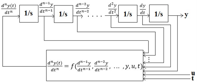
Simulink allows simulation of linear time-invariant (even nonlinear or time-varying) differential equations that can be written in an explicit form given by:
The corresponding block-scheme (to be designed in Simulink) is as shown in Fig. 1.
Fig. 1The integrator block scheme for solving differential equations in Simulink
In order to determine a linear dynamic system’s time response that depends on initial conditions and the system input, a set of mathematical equations representing the system is derived. For some simple systems, a closed-form analytical solution can be easily obtained. But for most of the systems (including nonlinear systems or those subject to complicated inputs), an integration must be carried out numerically to determine the output response that represents how the state of a dynamic system changes in time when subjected to a particular input. Simulink/MATLAB provides all useful resources for calculating time responses to several types of inputs.
As the derived equations consist of differential equations, an integration is required to be performed in order to determine a time response of the system. The integrator block with 1/ as the block symbol available in Simulink library is used to calculate the integral of the signal provided at the input i.e. left side of the block [14-15]. While solving a differential equation, the major task to perform includes integrating a given equation so as to get back the function without employing the derivative function. Integration of the derivative of a function is equal to the function itself. The integrator block serves the same purpose in the Simulink model. Simulink integrator blocks used in a block diagram are equal to an order of the differential equation that is being analyzed i.e. for solving a first order differential equation, only one integral block is needed, whereas for a second order differential equation, the number of blocks dragged and dropped into the model is two.
2.3. Transfer function approach
Simulink can also solve ordinary differential equations by defining systems using transfer functions, and thereby using techniques for numerical integration. Simulink has a standard block called the Transfer Fcn block which allows the direct input of numerator and denominator terms of the transfer function describing a given dynamic system. The Transfer Fcn block has a default form of first-order in the denominator () which can be modified for the specified different order for the numerator and denominator polynomials by entering coefficients associated with the respective polynomials (zero coefficient of the missing term must be included).
Any linear system can be characterized using a transfer function , which is an operator that takes an input to the output . For a continuous time system, system transfer function is essentially a ratio between Laplace transform of the output response of a system and Laplace transform of the input forcing function i.e. . The transfer function for any system can be obtained by taking a Laplace transform of the differential equation representing the given system with all initial conditions set to zero, and then solving the output response in terms of a given input forcing function with a factor multiplying taken out as the desired transfer function [2]. The desired transfer function is defined in Simulink by including coefficients of the polynomials in numerator and denominator of the transfer function as the inputs to the Transfer Fcn block in the Num and Den fields, respectively. This can be done by accessing the Function Block Parameter box where all information about the system can be entered within one block i.e. the Transfer Fcn block.
Now, the target is how to solve differential equations having non-zero initial conditions using transfer function approach. The paper presents two ways for resolving this issue (Section 3).
2.4. State space approach
A system in its state space representation replaces an th order differential equation with a single first-order matrix differential equation. The method is convenient for breaching a higher-order differential equation into sequences of first-order equations so that they can be easily solved using a matrix method. In order to model a second-order ODE using state space, the equation is broken down into two first-order state equations [16-18]. This can be achieved by allocating a subscripted variable for each state of the system in an order of increasing derivatives which includes letting , , and. This allows a re-statement of the equation in terms of state variables only.
To begin, select the State-Space block from the Continuous sub-menu of the Simulink library.
At this point the model is very general, and an equation of any order can be set up for solution in the block parameters. The equation inside the State-Space block is , . This represents the basic state-space equation, where = a vector of the first-order state variables, = output vector, = the state variable vector, = a forcing input function, = the state matrix, = input matrix, = output matrix, and = transmission matrix.
3. Results
Initial Value Problem (IVP) is an ordinary differential equation together with an initial condition which specifies the value of an unknown function at a given point in a time domain. Modeling a system in science related fields frequently requires solving an initial value problem.
For solving a differential equation given by Eq. (2) using integrator-based approach, first step is to rearrange the given differential equation such that the highest order derivative appears on the left-hand side while all the remaining terms appear on the right-hand side:
Thus, rearrange Eq. (2) in such a way that the highest differential term is separated from the other terms as shown below:
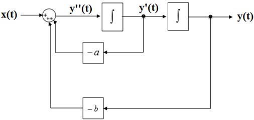
The corresponding integrator block-scheme (to be built in Simulink) is shown in Fig. 2.
In the paper, an initial value problem differential equation taken for the analysis is as follows:
Fig. 2Simulink model based on integrator block scheme
3.1. Integrator method
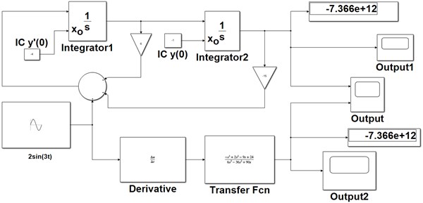
For solving Eq. (4) using integrator based approach, first step is to rearrange the given differential equation. Keep the highest order derivative on the left-hand side, and move all the remaining terms on the right-hand side. The resulting equation can be simulated in Simulink as shown in Fig. 3. The initial conditions specified at zero time instant i.e. 0 can be entered easily in the Integrator block.
Fig. 3The Simulink circuit model using integrator and transfer function (method 1)
Simulink (a MATLAB component) is very useful for simulating dynamic systems using a block-diagram model based approach [19]. A block diagram is simply a graphical representation of a process (which is composed of an input, the system, and an output). Thus, an interconnection of blocks in Simulink represents the system’s mathematical model. The lines interconnecting the blocks represent the variables describing the system behavior. The Display Sink block is a digital readout of an input signal at a current simulation time (the specified simulation stop time). The Scope Sink Block is used to display a signal as a function of time in a Simulink model. The term model refers to a set of mathematical equations representing a physical system, and thereby relates the system’s output signal to its input signal.
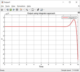
The simulated output after running simulation from 0 to 10 is shown below in Fig. 4. The Display Sink block is showing the numerical output value of IVP given by Eq. (4) at a time instant equal to 10 s (the specified current simulation stop time). Sampling issues must be taken care of while running a simulation in Simulink (a front-end tool designed for solving ordinary differential equations numerically). If the variable-step solver option is selected, the maximum step size parameter in the Max Step Size field box present in the Configuration Parameters window should be set to a lower value for better simulation results.
Fig. 4The simulated output using integrator method
3.2. Transfer function method
For using transfer function approach, take Laplace of Eq. (4). While writing the Laplace, following properties should be used:
The Laplace transform of Eq. (4) after plugging in the initial conditions becomes:
After solving for and combining into a single term, gives:
or
The analytical solution can be computed by applying partial fraction method on Eq. (8), and then taking inverse Laplace transform of the terms obtained after doing partial fraction decomposition [20]. The exact solution comes out to be:
Now, the target is how to solve it digitally using circuit simulation.
3.3. Method 1
3.3.1. The newly developed first way for solving Eq. (8) using transfer function in Simulink (method 1)
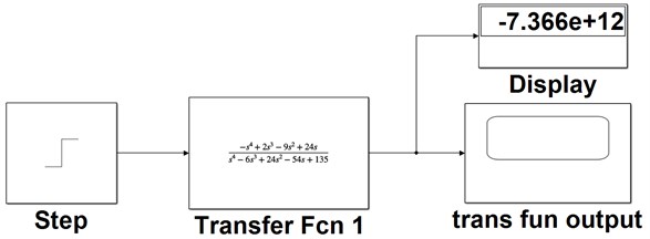
Take the factor multiplying the Laplace of an input function i.e. the multiple of as the transfer function. Thus, the transfer function to be entered in a Simulink Transfer Fcn block becomes equal to as follows:
The above transfer function can be re-written as:
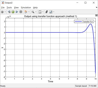
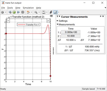
The transfer function can be implemented in Simulink by using a Derivative block in series with a Transfer Fcn block as shown in Fig. 3. The simulated output result of the above stated transfer function (method 1) by implementing Eq. (12) is shown below in Fig. 5.
Fig. 5The Simulated output with the transfer Fcn block using the method 1
3.3.2. Comparison of the simulated outputs using two different approaches
Figs. 6 and 7 display the values of the simulated output for time instants 0 s and 10 s using integrator and transfer function (method 1), respectively.
The simulated outputs for time instants 0 s and 10 s using integrator approach are –1 and –7.366×10¹², respectively.
The simulated outputs for time instants 0 s and 10 s using integrator approach are 0 and –7.366×10¹², respectively.
3.4. Method 2
3.4.1. The newly developed second way for solving Eq. (8) in Simulink (method 2)
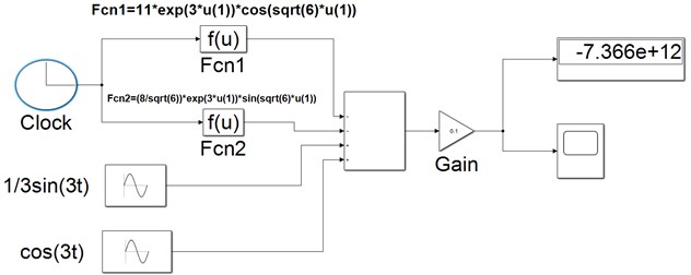
Take the factor multiplying the Laplace of a unit step function as the transfer function. Now, implement the transfer function as shown in Fig. 8.
Fig. 6The simulated output values for time instants t= 0 s and t= 10 s using an integrator scheme
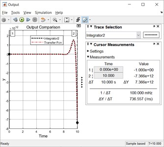
Fig. 7Outputs for t= 0 s and t= 10 s using the Method 1 (based on transfer function)
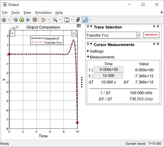
Fig. 8The Simulated model with the transfer Fcn block employing the method 2
By default, the Step block’s step time (time, in seconds, when an output steps/changes from the Initial value parameter to the Final value parameter) is 1. Also, the Initial value parameter (the block output until the simulation time reaches the Step time parameter) is 0 by default whereas, the Final value parameter (the block output when the simulation time reaches and exceeds the Step time parameter) is 1 by default.
Fig. 9 shows the output using a second way of employing transfer function approach (method 2).
The simulated outputs for time instants 0 s and 10 s using integrator approach are –1 and –7.366×10¹², respectively.
Fig. 9The simulated output with the transfer Fcn block using the method 2
3.4.2. Exact output
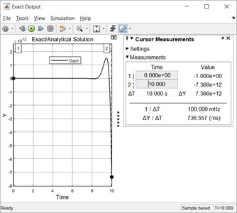
The analytical solution given by Eq. (10) can be simulated as shown in Fig. 10.
Fig. 10The simulated model for generating an exact output of Eq. (10) using analytical solution
The Clock Source Block is used in the Simulink model shown in Fig. 10 for generating a signal equal to the current time in the simulation. The Simulated exact output describing Eq. (10) is shown in Fig. 11.
Fig. 11The simulated exact output using an analytical solution
3.4.3. Output using state variable approach
Select the state variables for the Eq. (1). Choosing the state variables as successive derivatives, we get two first order differential equations as shown below:
These can be reorganized to obtain:
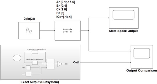
The Simulink model for simulating Eq. (15-16) using the State Space block is shown in Fig. 12. The block allows entering the direct input values of the A, B, C and D matrixes that are unique to a particular state-space model by going into the block parameter dialog box. The initial conditions are specified separately in a place to enter the ICs in the State Space block parameter window.
Fig. 12The model for comparing the state space solution with the exact solution
The model in state-space can be easily mapped in Simulink environment for numerical simulation. The simulated output using state space approach is presented in Fig. 13.
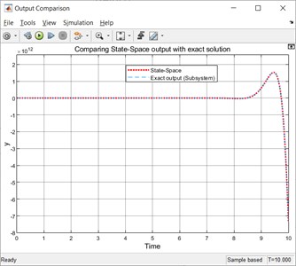
A comparison of the exact output with the state space based output is shown in Fig. 14. A spirit of comparing the simulation result with an analytical one is to ensure that a numerical approximation gives an acceptable result.
Fig. 13The simulated output using state space approach
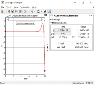
Fig. 14Comparison of the simulated exact output with the state space based output
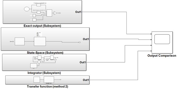
The Simulink model for comparing the outputs using an analytical approach, state space method, integrator method and transfer function approach (method 2) is shown in Fig. 15.
Fig. 15The model for comparing the outputs based on different approaches
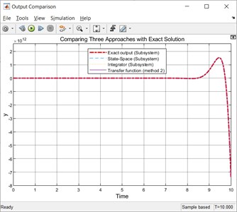
A comparison of outputs using an analytical method, state space method, integrator method and transfer function (method 2) using the analytical solution as a benchmark is shown in Fig. 16.
Fig. 16Comparing the simulated outputs
4. Conclusions
It can be concluded that the simulation results of initial value differential equation are in accordance with the analytical solution. Thus, the model based design can be related practically with real-time applications and Simulink can accurately predicts how the physical quantities related to a system change the system’s behavior. As Simulink enables the user to change the components to outfit any differential equation needed to be solved simply by changing the parameter values or adding or removing the blocks from the system model, therefore the software can be easily and more effectively employed for solving differential equations. Analyzing physical systems by building models and running them using the simulation software saves plenty of time and promote innovation in engineering and science related research fields.
References
-
Etter D. M., Engineering Problem Solving with MATLAB, Prentice Hall’s MATLAB Curriculum Series. Digitized, 2007.
-
Herman R. L., Solving Differential Equations Using Simulink. 2019.
-
Jain S., Modeling and Simulation Using MATLAB-Simulink. India: Wiley, 2011.
-
Roshen Tariq Ahmed Hamdi and Mahdi Ali Abdul Hussein, “Using Matlab-Simulink for solving differential equations,” Journal of Scientific and Engineering Research, Vol. 5, No. 5, pp. 307–314, Jun. 2018.
-
Longoria R. G., “Modeling and Simulation of using Matlab/Simulink,” University of Texas at Austin, Department of Mechanical Engineering, 2001.
-
Karris S. T., Introduction to Simulink® with Engineering Applications. Orchard Publications, 2006.
-
Karris S. T., Signal and System with MATLAB Computing and Simulink Modeling. Orchard Publications, 2007.
-
Aliyu B. Kisabo, Charles Osheku, Adetoro M. A. Lanre, and Aliyu Funmilayo A., “Ordinary differential equations: MATLAB/Simulink solutions,” International Journal of Scientific and Engineering Research, Vol. 3, No. 8, Jan. 2012.
-
Lambert J. D., Numerical Methods for Ordinary Differential Systems: The Initial Value Problem. Chichester: Wiley, 1992.
-
Mohindru P., MATLAB and SIMULINK (A Basic Understanding for Engineers) with Cambridge Scholars Publishing. England: Newcastle upon Tyne, 2020.
-
Nehra V., “Engineering simulation using graphical programming tool Simulink: putting theory into practice,” in National Conference on Contemporary Techniques and Technologies in Electronics Engineering, pp. 372–377, 2013.
-
V. Nehra, “MATLAB/Simulink based study of different approaches using mathematical model of differential equations,” International Journal of Intelligent Systems and Applications, Vol. 6, No. 5, pp. 1–24, Apr. 2014, https://doi.org/10.5815/ijisa.2014.05.01
-
Frank Pietryga, “Solving differential equations using Matlab/Simulink,” in Proceedings of the 2005 American Society for Engineering Education Annual Conference and Exposition, 2005.
-
https://kcir.pwr.edu.pl/~mucha/SciEng/lecture9.pdf
-
http://people.uncw.edu/hermanr/mat361/Simulink/ODE_Simulink.pdf
-
http://www.mathworks.com.
-
http://people.uncw.edu/hermanr/mat361/Simulink/StateSpace.pdf
-
https://www.uml.edu › State-Space_tcm18-190082
-
Sulaymon Eshkabilov, “MATLAB/Simulink applications in solving Ordinary Differential Equations,” Sep. 2013.
-
Math Notes, Paul Dawkins, http://tutorial.math.lamar.edu, 2018.
About this article

