Genetic engineering – construction of a network of arbitrary dimension with periodic attractor

1. Introduction

Genetic engineering started 39 years ago at the Miami Winter Symposium, where three independent groups described Agrobacterium tumefaciens-mediated genetic transformation, leading to the production of normal, fertile transgenic plants [1].

Genetic engineering is a modern area of biotechnology that combines knowledge and techniques from a whole block of related sciences. It is the process of changing an organism’s DNA to introduce new, desirable traits. Many organisms, from bacteria to plants and animals, have been genetically modified for academic, medical, agricultural, and industrial purposes.

Genetic regulatory network (GRN) is responsible for many important functions of living organisms. It exists in any in any cell of any living organism. Huge amounts of experimental data are stored and need systematization and research. One the effective way of treating this is to consider the mathematical models of GRN. If they are appropriate and exhibit sufficient correspondence with experimental information, they (models) can be used for understanding, managing and control over GRN. We focus on models formulated in terms of dynamical systems. Dynamical systems, used for modeling GRN, consist of ordinary differential equations of special structure. Look at the system below.

Consider the general form of writing the $n$-dimensional dynamical system, that is expected to model a genetic regulatory network:

where ${\mu }_k>0$, ${\theta }_k$ and $v_k>0$ are parameters, and $w_{ij}$ are elements of the $n\times n$ regulatory matrix $W$. The parameters of the GRN have the biological interpretations [2,3].

In the system Eq. (1) the sigmoid logistic function $f\left(z\right)=\frac{1}{1+e^{-\mu z}}$ is used [4].

It is to be mentioned, that first system of this form was used to model populations of neurons [5], [6]. There were attempts to use systems of the form Eq. (1) for the creation of Virtual Network Topology to manage traffic in telecommunication networks [7]. It is recommended also to be acquainted with the articles [8], [9] on the subject.

In this article, we would like to consider the construction of models of GRN with the required properties. Due to the restricted volume of the conference proceedings, we will discuss the creation of models of any dimensionality, considering bounded periodic attractor. Solutions, tending to periodic attractors, reflect rhythmical processes in organisms. Our plan is the following. First, we consider the three-dimensional system of ordinary differential equations of the form Eq. (1) and show, that it has a stable periodic trajectory, which serves as an attractor for other trajectories. Then we construct a greater system, which consists of three-dimensional systems. The periodic attractors in any of three-dimensional systems, when combined in higher dimensional phase space, produce a periodic attractor of a higher dimension.

2. Two-dimensional systems

The two-dimensional system of the form Eq. (1) is defined, if all the parameters are given. Consider $v_1=v_2=$ 1; ${\mu }_1=$ 20, ${\mu }_2=$ 40; ${\theta }_1=$ 1, ${\theta }_2=$ –0.3. The coefficients $w_{ij}$ are elements of the matrix $W$and behavior of solutions depends on it.

Consider the system Eq. (1) with regulatory matrix:

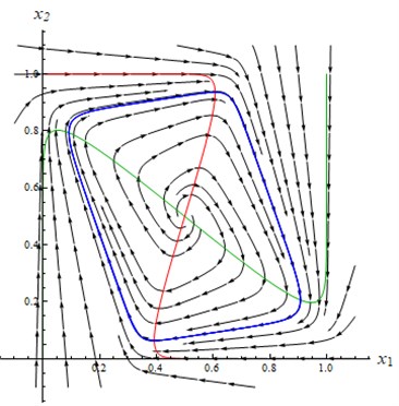
The nullclines of the system Eq. (1) together with the stable periodic solution are depicted in Fig. 1 [10].

Fig. 1The nullclines x1 – red, x2 – green

There is a unique critical point at (0.5; 0.5). The characteristic equation for equilibria (0.5; 0.5) is:

where $B=$ –7, $C=$ 62. Solving the equation we have ${\lambda }_{\mathrm{1,2}}=$ 3.5±7.05. The type of equilibria is an unstable focus.

3. Three-dimensional systems

The three-dimensional system of the form Eq. (1) is defined, if all the parameters are given. Consider $v_1=v_2=v_3=$ 1; ${\mu }_1={{\mu }_2=\mu }_3=$ 4; ${\theta }_1=$ 4, ${\theta }_2=$ 0, ${\theta }_3=$ 0. The coefficients $w_{ij}$ are elements of regulatory matrix $W$ and behavior of solutions depends on it.

Consider the system Eq. (1) with regulatory matrix:

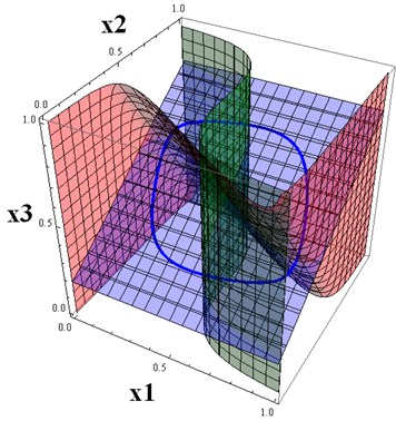
The nullclines of system Eq. (1) together with the stable periodic solution are depicted in Fig. 2. There is a unique equilibria at (0.5; 0.5; 0.5). The central location of the critical point is due to the special choice of the parameters ${\theta }_i$.

Fig. 2The nullclines x1 – red, x2 – green, x3 – blue and the periodic trajectory

The characteristic equation for the critical point (0.5; 0.5; 0.5) is:

where $A=$ –1, $B=$ 3, $C=$ –13. Solving the equation we have ${\lambda }_{\mathrm{1,2}}=$ 1.102±1.6866; ${\lambda }_3=$ –3.20. The type of critical point is an unstable saddle-focus.

In fact, we have provided an example of the 3D system without stable critical points. More examples of this kind were obtained in the paper [11].

4. Six-dimensional systems

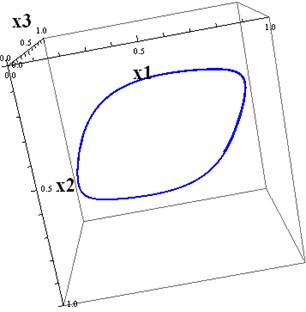
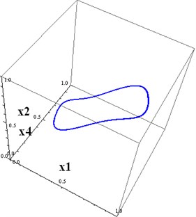
We are able now to construct systems of any dimensions, combining the above two- and/or three-dimensional systems. Let us construct six-dimensional system with a periodic attractor, combining two identical three-dimensional systems. Consider 6 by 6 block matrix $W$, where the 3 by 3 matrix Eq. (4) is placed at the left-upper and right-lower corners. Other spaces are filled by zeros. The resulting system of the form Eq. (1) describes a GRN with 6 elements and it has the six-dimensional periodic attractor. We can visualize three-dimensional projections of this attractor on subspaces.

The initial conditions for a solution of the six-dimensional system, tending to a six-dimensional periodic attractor, are:

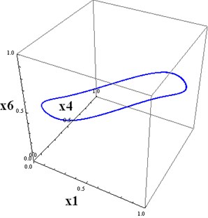
Fig. 3a) The projections of 6D trajectories to 3D subspace(x1,x2,x3) (it is solution of the base three-dimensional system), b) The projections of 6D trajectories to 3D subspace (x1,x2,x4)

a)

b)

Fig. 4a) The projections of 6D trajectories to 3D subspace (x1,x4,x6), b) The projections of 6D trajectories to 3D subspace (x2,x3,x6)

a)

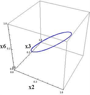
b)

Fig. 5a) The projections of 6D trajectories to 3D subspace(x1,x5,x6), b) The projections of 6D trajectories to 3D subspace (x3,x4,x5)

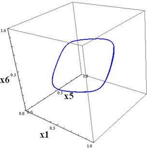
a)

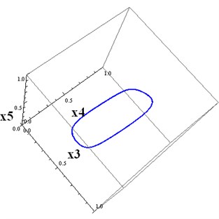
b)

5. Conclusions

Periodic attractors can be constructed for higher-dimensional systems of the form Eq. (1), using known periodic trajectories for low-dimensional systems. In our example, we first constructed the three-dimensional system with a regulatory matrix Eq. (4). Then we constructed the six-dimensional square matrix with two blocks on the main diagonal, consisting of the matrix Eq. (4). Other parameters are chosen as for the three-dimensional case. Then we computed the solution of the six-dimensional system with the above initial conditions. This trajectory, projected on $(x_1,x_2,x_3)$, tends to the three-dimensional projection of the attractor. This trajectory, projected on $(x_4,x_5,x_6)$, tends to the three-dimensional projection of the attractor onto the subspace $(x_4,x_5,x_6)$. The initial conditions for these projections, differ. This is why Fig. 4(a) and Fig. 5(a) are not identical.

It is possible, proceeding in this way, to construct attractors for any dimension. In the second section, the two-dimensional system is provided, which has a stable periodic solution. A periodic attractor, therefore, can be constructed for any dimension, combining two and three dimensional blocks in the main regulatory matrix $W$ (for example, 4 = 2 + 2, 5 = 3 + 2, 6 = 3 + 3 = 2 + 2 + 2, etc.). In particular, the six-dimensional attractor can be constructed by combining three independent two-dimensional systems.

The situation is different if we combine the six-dimensional system with two three-dimensional systems, which have stable periodic solutions, but with different periods. Recall, that in our example periods for solutions of both three-dimensional components are the same since the three-dimensional systems are identical. The attractor in a resulting six-dimensional system must exist, but it should be a chaotic subset of the phase space, formed by non-periodic six-dimensional trajectories. It is like Lissajous figures, where the periods are incommensurable.