Genetic engineering – construction of a network of four dimensions with a chaotic attractor

1. Introduction

In 1944 DNA was discovered as a universal genetic material. After ten years, its molecular structure studied. Thus began the era of DNA science and technology [1]. The term genetic engineering appeared at the turn of the 70s of the twentieth century. Genetic engineering is not a separate science. It is a large and constantly developing scientific and technological platform. It has absorbed the most valuable from genetics, biochemistry, chemical engineering, molecular and cellular biology, microbiology, and virology.

We wish to describe the transformation and the construction, not the DNA itself, but combinations of genes, expressing proteins and forming the genetic regulatory network (GRN in short). GRN is being explored in biochemistry, neurobiology, ecology, and engineering. Gene regulatory networks are mathematical and computational models describing the logic underlying the regulatory occurrences among genes while a specific cell program is operating [2]. GRN is a group of genes coordinated the functioning of which ensures the formation of a certain phenotypic sign of an organism. One of the methods to describe the GRN is to use a system of nonlinear differential equations.

We consider the system of nonlinear differential equations, where in focus is chaos and a chaotic attractor. The study of the concept of chaos is very relevant in our time because with the help of this concept many phenomena in various fields of science and everyday life are explained. Deterministic chaos combines determinism and randomness, limited predictability and unpredictability, and manifests itself in different phenomena such as the kinetics of chemical reactions, the turbulence of liquid and gas, geophysical, in particular, weather changes, physiological reactions of the body, population dynamics and epidemics. Computer visualization of chaotic attractors reveals them complexity and unusual configurations in three-dimensional space.

Consider the general form of writing the n-dimensional dynamical system that models a genetic regulatory network:

where ${\mu }_i>0$, ${\theta }_i$ and $v_i>0$ are parameters, and $w_{ij}$ are elements of the $n\times n$ regulatory matrix $W$. The parameters of the GRN have the following biological interpretations: $v_i$ – the rate of degradation of the $i$-th gene expression product; $w_{ij}$ – the connection weight or strength of control of gene $j$ on gene $i$. Positive values of $w_{ij}$ indicate activating influences while negative values define repressing influences; ${\theta }_i$ – the influence of external input on gene $i$, which modulates the gene’s sensitivity of response to activating or repressing influences [3, 4]. The rate of increase in the expression level is given by the sigmoidal logistic function $f\left(z\right)=\frac{1}{1+e^{-\mu z}}$ [5].

2. Four dimensional systems

The four-dimensional system of the form Eq. (1) is defined, if all the parameters are given. Let $v_1=v_2=v_3=v_4=$ 1; ${\mu }_1={\mu }_2={\mu }_3={\mu }_4=$ 10; ${\theta }_1=$ 1.2, ${\theta }_2=$ –0.7, ${\theta }_3=$ 1.8, ${\theta }_4=$ –0.28. The initial values $x_1\left(0\right)=$ 0.5, $x_2\left(0\right)=$ 0.32, $x_3\left(0\right)=$ 0.4, $x_4\left(0\right)=$ 0.39. The coefficients $w_{ij}$ are elements of the so called regulatory matrix $W$ and behavior of solutions heavily depends on it.

Consider the system Eq. (1) with the regulatory matrix:

This system consists of two independent two-dimensional systems. There is exactly one critical point. The standard linearization analysis provides the characteristic numbers ${\lambda }_{\mathrm{1,2}}=$ 0.2469±4.9875i; ${\lambda }_{\mathrm{3,4}}=$ 3.4667±4.9215i.

Change now two elements at the right upper $\left(w_{14}\right)$ and left lower $\left(w_{41}\right)$ corners. Let $w_{41}=$ 0.1 and $\left(w_{14}\right)$ values are listed in Table 1.

In the article for Lyapunov exponents calculation the package ‘lce.m for Mathematica’ was used [6]. Another Wolfram Mathematica program ‘Lynch-DSAM.nb’ was also used to check the correctness of Lyapunov exponents calculation [7].

Calculations showed the following:

1) $-1.2\le w_{14}<-1$ the system Eq. (1) with the regulatory matrix Eq. (2) has a periodic solution;

2) $w_{14}=$ –1 the system Eq. (1) with the regulatory matrix Eq. (2) has a chaotic solution;

3) $-0.9\le w_{14}<-0.7$ the system Eq. (1) with the regulatory matrix Eq. (2) has a periodic solution;

4) $w_{14}=$ –0.7 the system Eq. (1) with the regulatory matrix Eq. (2) has a chaotic solution;

5) $-0.6\le w_{14}<-0.4$ the system Eq. (1) with the regulatory matrix Eq. (2) has a periodic solution.

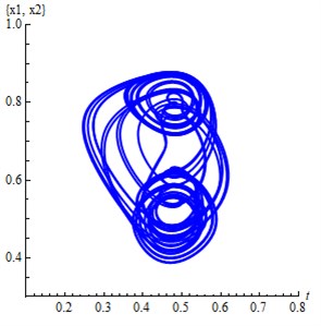
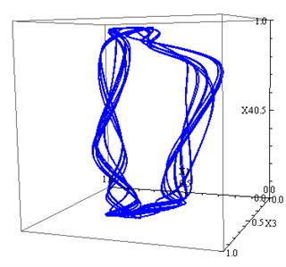
Fig. 1a) The projection of the attractor Eq. (2) on 2D subspace (x1, x2), b) The projection of the attractor Eq. (2) on 3D subspace (x1, x2,x4)

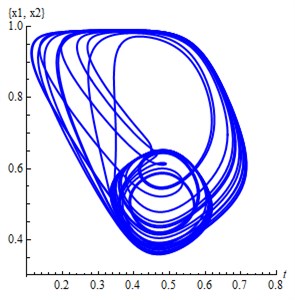
a)

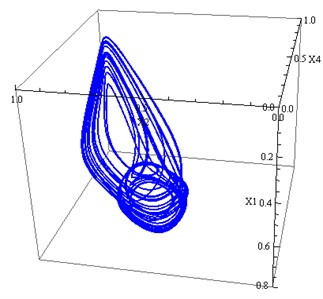
b)

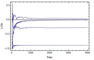
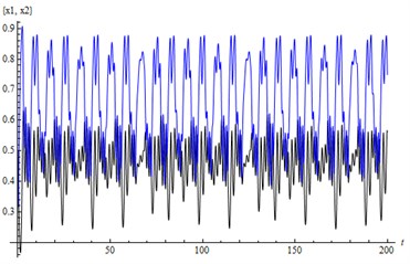
Fig. 2a) LE1, LE2, LE3, LE4= (0.05, 0, –0.88, –0.99) – a chaotic attractor, b) solutions (x1, x2)

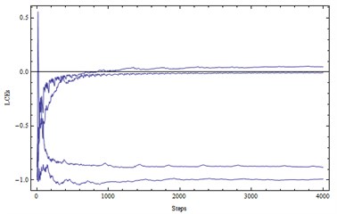
a)

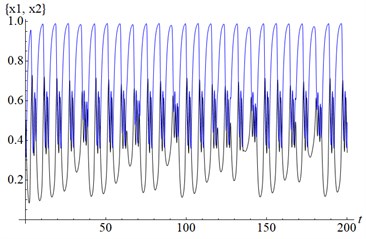
b)

For $w_{14}=$ –1 there is exactly one critical point (0.4823; 0.6802; 0.5534; 0.4085). The characteristic equation for critical point (0.4823; 0.6802; 0.5534; 0.4085) is:

where $A=$ –7.21, $B=$ 60.35, $M=$ –163.60, $L=$ 776.41. Solving the equation we have ${\lambda }_{\mathrm{1,2}}=$ 0.22±4.67 and ${\lambda }_{\mathrm{3,4}}=$ 3.38±4.91. The type of critical point is an unstable focus-focus.

For $w_{14}=$ –0.7 there is exactly one critical point (0.4805; 0.6190; 0.5533; 0.4086). The characteristic equation for critical point (0.4805; 0.6190; 0.5533; 0.4086) is Eq. (3), where $A=$ –7.30, $B=$ 62.64, $M=$ –178.92, $L=$ 842.35. Solving the equation we have ${\lambda }_{\mathrm{1,2}}=$ 0.25±4.86 and ${\lambda }_{\mathrm{3,4}}=$ 3.40±4.90. The type of critical point is an unstable focus-focus.

Fig. 3a) The projection of the attractor Eq. (2) on 2D subspace (x1, x2), b) The projection of the attractor Eq. (2) on 3D subspace (x1, x3,x4)

a)

b)

Fig. 4a) LE1, LE2, LE3, LE4= (0.03, 0, –0.26, –0.89) – a chaotic attractor, b) solutions (x1, x2)

a)

b)

3. Conclusions

Various fields of science, including biology, need mathematical models that offer a convenient analysis of dynamic processes in GRN and their collective behavior to understand, predict and control regulatory mechanisms. That is why modeling genetic networks is a necessary part of our investigation. Mathematical models are needed to suppress tumors since it is important to understand how the system behaves and behavior changes. The same system with different parameters can have periodic or chaotic solutions. A stable fixed point is also possible. In this article, a stable point is not considered since this is the simplest state of the system. We are interested in a chaotic and periodic solution for the therapy of various diseases such as blood cancer. Attractors of dynamical systems describe the future states of GRN. Attractors of high-dimensional systems can be of different structures: periodic or chaotic attractors.

References

-
M. Pyne, K. Sukhija, and C. P. Chou, “Genetic Engineering,” Comprehensive Biotechnology, Vol. 2, pp. 81–91, 2011, https://doi.org/10.1016/b978-0-08-088504-9.00089-1
Paolo Tieri and Filippo Castiglione, “Modeling macrophage differentiation and cellular dynamics,” Systems Medicine, Vol. 2, pp. 511–520, 2021.
N. Vijesh, S. K. Chakrabarti, and J. Sreekumar, “Modeling of gene regulatory networks: A review,” Journal of Biomedical Science and Engineering, Vol. 6, No. 2, pp. 223–231, 2013, https://doi.org/10.4236/jbise.2013.62a027
I. Samuilik and F. Sadyrbaev, “Modelling three dimensional gene regulatory networks,” WSEAS Transactions on Systems and Control, Vol. 16, pp. 755–763, 2021.
E. Brokan and F. Z. Sadyrbaev, “On attractors in gene regulatory systems,” Proceedings of the 6th International Advances in Applied Physics and Materials Science Congress and Exhibition: (APMAS 2016), Vol. 1809, No. 1, p. 020010, 2017, https://doi.org/10.1063/1.4975425
“MATLAB Software,” www.msandri.it/soft.html.
S. Lynch, Dynamical Systems with Applications Using Mathematica. Springer, 2017.
Cited by
About this article
ESF Project No. 8.2.2.0/20/I/ “Strengthening of Professional Competence of Daugavpils University Academic Personnel of Strategic Specialization Branches 3rd Call”.