On the issue of the motion of balls in a double pendulum

1. Introduction

During the acceleration and deceleration of the rotor in the ball autobalancer, an intense collision of freely moving balls occurs. This interaction between the balls obviously affects the transient processes of the rotor. At the same time, the influence of impacts between the balls has not been studied enough due to the transience of the process of acceleration of the rotor and the nature of the movement and impact of the balls that is difficult to describe. When the balls collide with each other, their elastic deformation occurs [1]. The kinetic energy of the balls is partly converted into the potential energy of deformation and partly into the internal energy of the body, which causes an increase in the temperature of the balls. Most publications [2-7] consider transient modes in auto-balancing devices (ABD) with the ability of balls to pass through each other without taking into account impacts between them.

Also known is the Kapitsa pendulum model with a suspension point oscillating in a vertical plane, described in [7, 8]. However, these papers do not consider the double pendulum and the impact of the ball on the obstacle. In [11], a mathematical model of a double pendulum with a rotating and oscillating suspension point was obtained and the conditions for numerical simulation of ball collisions were obtained.

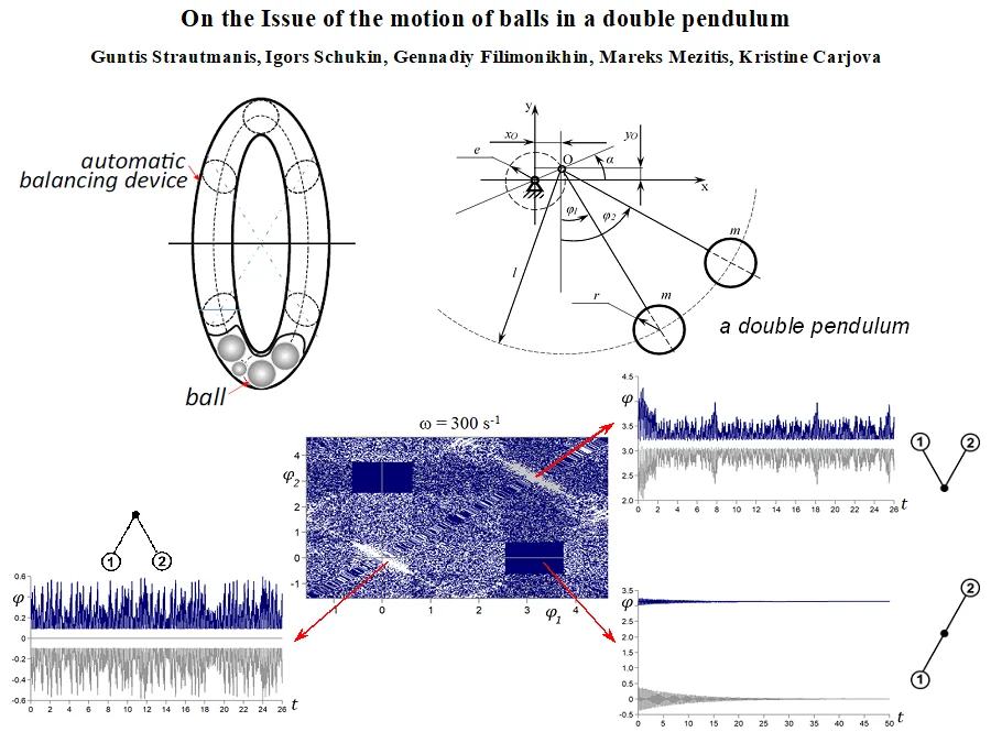
In this paper, we consider a double pendulum of identical balls, which are fixed on rigid links with one common suspension point. When the pendulums oscillate between the balls, a shock occurs, which can be both elastic and absolutely inelastic. In the case of an elastic impact, sticking of the balls is possible, as a result of which the double pendulum system begins to behave like a single pendulum. The suspension point of the pendulums oscillates in a vertical plane or makes rotational movements.

2. Mechanical model of double pendulum

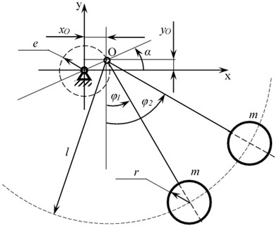
The physical model of a double pendulum with a moving suspension point is shown in Fig. 1. Balls have the same mass $m$ and radius $r$, suspended on an inextensible rigid thread of length $l$. The suspension point of the balls can remain at rest or make circular motions in a vertical plane along a trajectory in the form of a circle of radius $e$, while a dissipative moment acts at the suspension point of the pendulums, with a dissipation coefficient $b$.

Fig. 1Calculation scheme of a double pendulum with a rotating suspension point

The differential equations of motion of a system of pendulums with unsteady motion of the suspension point of the balls were obtained in [11] and have the form:

If we assume that the suspension point of the pendulums O rotates at a constant velocity, i.e. the motion of the suspension point is fixed ($\ddot{\alpha }=0;\dot{\alpha }=\omega =$ const, $\alpha =\omega t$), then the equations of motion will take the form [11]:

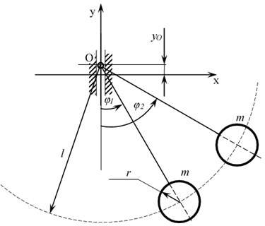
Systems of pendulums with a suspension point oscillating with a constant angular velocity in the vertical direction are shown in Fig. 2. After carrying out all the transformations, we obtain a system of differential equations consistent with the Kapitza equation [7, 11]. For pendulums with an oscillating suspension point in the presence of dissipation in it, the equations take the form:

The following models of pendulums are considered in the work:

1. Kapitza pendulum for different values of viscous friction at the suspension point (in the traditional model of the Kapitza pendulum, the coefficient of viscous friction at the suspension point is 0);

2. Double Kapitza pendulum for different values of viscous friction at the suspension point and recovery coefficient $k_d=$ 0.8 [11] (not quite elastic impact is considered).

To take into account various possible modes and forms of motion of the balls (impact or sticking together of the balls), in this work, we used a modified method for the numerical solution of Runge-Kutta differential equations [10, 11]. After each step of numerical integration, the phase coordinates were checked and corrected in the case of bodies sticking together. This approach also takes into account the possibility of separation of the balls under the influence of external forces during further movement.

Fig. 2Calculation scheme of a double pendulum with an oscillating suspension point

3. Results of numerical simulation

At the first stage, one differential Eq. (5) is considered with the following parameters of the pendulum: $l$= 1,0 m – the distance from the suspension point to the centre of the ball; $r$= 0,1 m – the radius of the ball; $g$ = 9,81 – free fall acceleration; $e$ = 0,1 m – the amplitude of the oscillation of the suspension point; $b$ = (0…0,2) – dissipation coefficient at the suspension point; $\omega$ = (50…314,15) s^-1 – the angular velocity of the oscillatory movement of the suspension point.

3.1. Results for absolutely inelastic impact

On Fig. 3 shows the region of attraction of the ball motion modes for different values of the angular velocity of the oscillation of the suspension point at $b$ = 0,2.

Fig. 3Area of attractions for two equilibrium states: dark regions – initial conditions (φ0, φ˙0) lead to upper position of the ball (φ = π), white – lead to lower position of the ball (φ = 0); a) parameters: b = 0.2; ω = 314.15 s-1; b) parameters: b = 0.2; ω = 50 s-1

a)

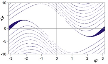
b)

On Fig. 4 shows the time sweep for various initial parameters of the pendulum motion. As follows from Fig. 4(a), when choosing the initial coordinate and velocity of the ball in the dark zone of the attraction region (Fig. 3), the pendulum moves in an inverted state. When choosing the initial conditions in the bright zone of the attraction region (see Fig. 4(b)), the pendulum oscillates in the lower position.

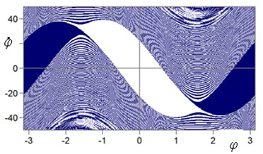
When the dissipation coefficient at the suspension point decreases to zero ($b=$ 0), along with the indicated modes, another mode of motion of the ball arises – continuous rotation of the ball around the suspension point. On Fig. 5 shows the region of attraction of the ball motion modes for various values of the angular velocity of the oscillation of the suspension point at $b=$ 0.

Fig. 4Transient process to equilibrium state: a) φ0= 2.45; φ˙0= 0; b) φ0= 2.5; φ˙0= 0. Parameters: b= 0.2; ω= 50 s-1

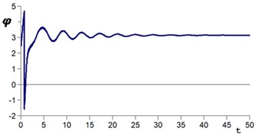
a)

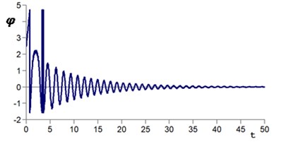
b)

Fig. 5Area of attractions for three steady states: dark regions – initial conditions (φ0, φ˙0) lead to upper equilibrium state (φ = π), white – to lower equilibrium state (φ = 0), gray – to rotation; a) parameters: b= 0; ω= 314.15 s-1; b) parameters: b= 0; ω= 50 s-1

a)

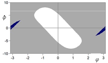
b)

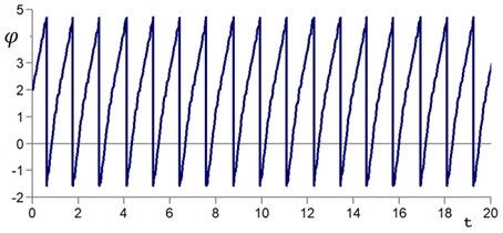
On Fig. 6 shows the time sweep when choosing the initial parameters of the pendulum motion in the gray zone of the attraction region (see Fig. 5). As follows from this figure, the pendulum will continuously rotate around the suspension point. When choosing the initial coordinate and velocity of the ball in the dark zone of the attraction region (Fig. 5), the pendulum moves in an inverted state. When choosing the parameters in the light zone of the attraction region, the pendulum oscillates in the lower position.

Fig. 6Rotation regime from initial conditions φ0= 2; φ˙0= 0. Parameters: b= 0; ω= 50 s-1

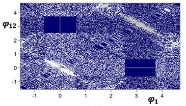
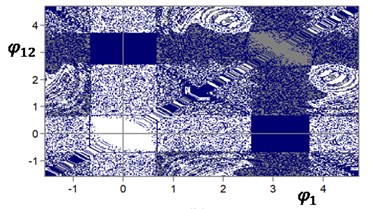
In the numerical simulation of differential Eqs. (5-6) for a double pendulum with an oscillating suspension point, the regions of attraction of the modes of motion of the pendulums at different angular velocity of the oscillation of the suspension point are constructed, shown in Fig. 7.

Fig. 7Area of attractions for three steady states: dark regions – initial conditions (φ˙1= 0; φ˙2= 0) lead to equilibrium state (φ1,2=π; φ2,1=0), white – to oscillations around lower position, gray – to oscillations around upper position. Parameters: a) b= 0.2; ω= 300 s-1; b) b= 0.2; ω= 150 s-1

a)

b)

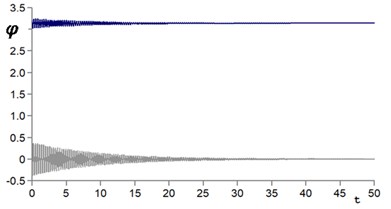
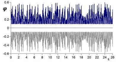
Fig. 8Time histories of pendulum oscillations (φ˙1=0; φ˙2=0) dark line – body 1, grey – body 2: a) φ1= 3.2; φ2= –0.2; b) φ1= 0.2; φ2= –0.2; c) φ1= 3.7; φ2= 2.6. Parameters ω= 300 s-1; b= 0.2

a)

b)

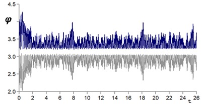
On Fig. 8 shows the time sweep for various initial parameters of the pendulum motion. As follows from Fig. 8, when choosing the initial coordinate and speed of the ball in different zones of the attraction area (Fig. 7), the pendulums move in different states: opposite, in the lower one with impacts, and inverted with impacts between the balls.

4. Conclusions

Based on the system of differential equations obtained by the authors for a pendulum system with a rotating and oscillating suspension point, the problem of numerical simulation with instantaneous interaction of balls (impact) is considered.

The result is obtained that the size of dissipation in the suspension affects the motion of the balls. With a decrease in the dissipation value, the regime zone expands, in which the balls continuously rotate around an axis passing through the suspension point.