Abstract
Ice will form in winter in high-latitude areas of China. As the external temperature rises, the ice cover will generate thermal expansion force on the restrained object. Based on the single-factor sensitivity method, the thermal solid coupling model is used to calculate the ice layer thermal stress. The intensity of the water quality monitoring system in China's high latitude icing period is modeled and calculated. The results show that with the increase of the external temperature rise rate, the external initial temperature decreases and the thickness of the ice layer increases, the expansion force of the ice layer temperature increases, and the stress field of the ice layer presents nonlinear distribution. The extreme point is located at 1/3 of the ice layer thickness. The water quality monitoring system will produce high stress at the edge of the body, which should be paid attention to when it is concentrated on engineering use.
Highlights
- Based on the single-factor sensitivity method, take advantage of finite element analysis software, the Thermosolid coupling method. The effects of external ambient temperature, environmental temperature rise rate, ice thickness on the ice temperature field, and temperature expansion force were analyzed.
- With the increase of the external temperature rise rate,the external initial temperature decreases and the thickness of the ice layer increases, the expansion force of the ice layer temperature increases, and the stress field of the ice layer presents nonlinear distribution. The extreme point is located at 1/3 of the ice layer thickness.
- Extrusion effect of temperature expansion force on the water quality monitoring system was analyzed, the water quality monitoring system will produce high stress at the edge of the body, which should be paid attention to when it is concentrated on engineering use.
1. Introduction
More than 75 % of China’s regions have frozen phenomenon [1], which is particularly common in high latitude regions, such as Heilongjiang, Inner Mongolia, Jilin, etc. [2]. From November to March of the next year, the river water will freeze. With the increasing solar radiation will cause the outside world to heat up, the vibration amplitude of hydrogen and oxygen atoms in the ice layer will increase, and the ice layer will expand. Due to the constraints on both sides of the river bank, the expansion of the ice layer will be limited. Therefore, thermal stress will be generated inside the ice layer. The research on the thermal expansion force of the ice layer has been started by scholars at home and abroad for a long time. Liu X. Z. placed a cryogenic pressure sensor on the ice layer that can be detected in real time and has static force, and analyzed the interaction between the ice layer and the structur kharik [3].Shang Jian et al. studied the expansion force of ice layer temperature and its influence on prestressed aqueduct, established a coupling model of ice aqueduct, and studied the change of expansion force of ice layer temperature under different ice layer thickness by using direct coupling and indirect coupling methods respectively [4]. Ansys software is used to analyze the water quality monitoring system under the effect of thermal expansion force of ice layer temperature, revealing the action law of the water quality monitoring system monitoring shell strength.
2. The constitutive model of ice
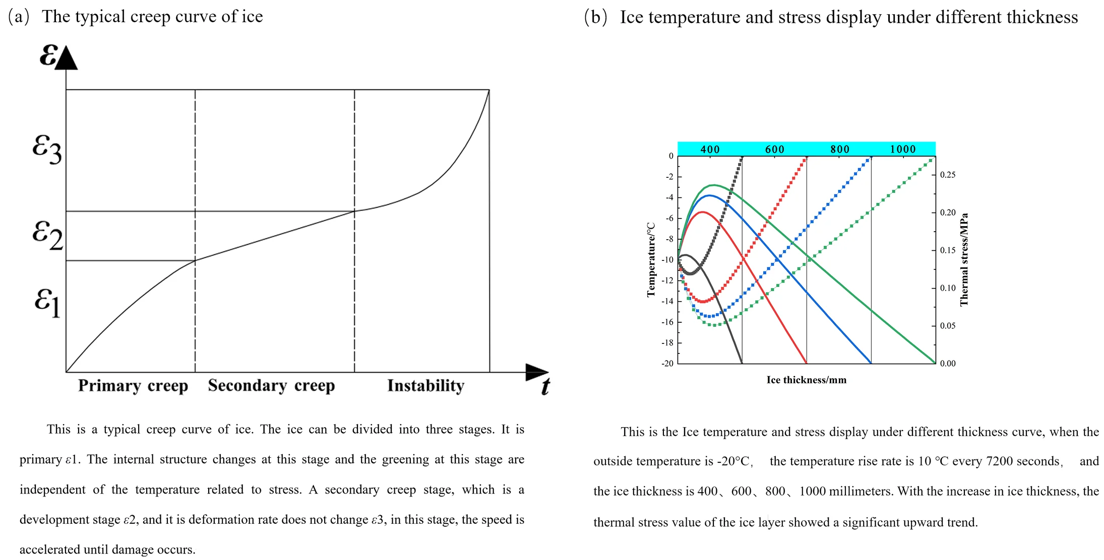
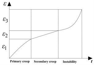
The typical creep curve of ice is as follows, as shown in Fig. 1. The ice can be divided into three stages. It is primary . The internal structure changes at this stage and the greening at this stage are independent of the temperature related to stress. A secondary creep stage, which is a development stage , and it is deformation rate does not change , in this stage the speed is accelerated until damage occurs.
Fig. 1The typical creep curve of ice
The creep of ice can be expressed as:
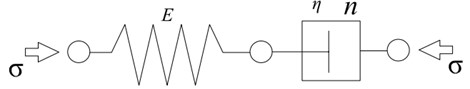
When calculating the thermal expansion force, most of the strains are a secondary creep. Its stress variation relationship can be shown by the viscoelastic model of ice shown in Fig. 2.
The temperature expansion force of the ice layer needs to calculate the temperature field of the ice layer first, and then solve the stress field distribution of the ice layer through the thermal solid coupling [5, 6, 7].
Fig. 2The viscoelastic model of ice, where E is the elastic modulus, η is viscosity index, n is stress index, σ is ice stress
3. Three dimensional geometric model of ice layer
In the surface water area, the length of the river is much larger than the width of the river. According to the detection of the Hydrological Bureau, the deepest knot in the surface water area is not up to one meter, establish a geometric model with a length of 20 m and width of 2 m. Define the path on the center line of the box. Hexahedral grids are used to divide the length direction of the geometric model. The grid size in the length direction is 1.0 meter, and the grid size in the width direction is 0.2 meters. In the thickness direction, the grid division size is 0.03 meters. The overall grid division and its central cutting interface are shown in Fig. 3.
Resin and ice material parameters are shown in Table 1.
Fig. 3Finite element model of ice layer
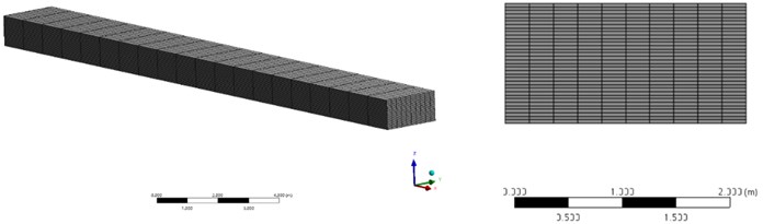
Table 1Resin and ice material parameters
Material | Elastic modulus / MPa | Poisson’s ratio | Density / (Kg·m-3) | Coefficient of thermal expansion / 10-5℃-1 | Thermal conductivity / (W·(m·℃)-1) |
Resin | 3120 | 0.39 | 1100 | 7.3e-5 | 0.20 |
Ice | 2300 | 0.35 | 1000 | 5.2e-5 | 0.64 |
4. Calculation of ice temperature field and stress field
The rate of temperature rise of the ambient temperature, the ambient temperature, and the ice layer thickness is the three factors that affect the temperature field and stress field of the ice layer [8, 9]. According to the single factor sensitivity method, Calculate the influence rule of three factors.
5. Analysis of the influence of external ambient temperature
Take the thickness of the ice layer as 1.0 meter, analyze this situation, and respectively give the initial temperature of the upper-end surface of the ice layer as –10 ℃, –15 ℃, and –20 ℃. Assuming that the initial temperature of the ice layer is evenly distributed. The external temperature rise rate is 10 ℃ every 7200 seconds. Impose fixed constraints on both sides of the geometric model, impose symmetrical constraints on the left and right of the ice layer, and do not impose any constraints on both sides of the ice layer thickness direction to simulate the growth effect of the natural expansion of the ice layer under natural conditions. the distribution of ice layer temperature field, cloud diagram and stress field cloud diagram is shown, as shown in Fig. 4 and Fig. 5(a), (b), (c) represents the cloud image display under –10 ℃, –15 ℃, –20 ℃. It can be seen that the lower the external temperature is, the greater the ice layer temperature expansion force.
Fig. 4Ice temperature field distribution

a)

b)

c)
Fig. 5Ice stress field distribution
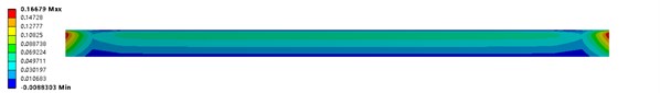
a)
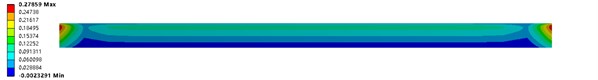
b)
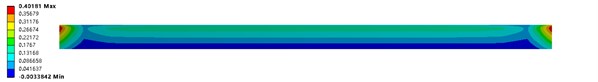
c)
6. Analysis on the effect of environmental temperature rise rate
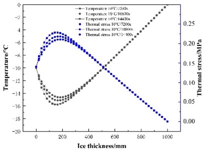
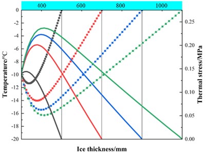
When the external environment is minus 20 ℃ and the ice thickness is 1.0 m, the environment temperature rise rate is controlled by the user-defined temperature rise function, which is respectively 10 ℃ of 7200 seconds, 10 ℃ of 14400 seconds, 10 ℃ of 18000 seconds. The Path node temperature and the thermal stress path of the ice layer temperature field obtained through numerical calculation are shown in Fig. 6. It can be seen that with the increase of temperature speed, the thermal stress value of ice layer is higher.
Fig. 6Ice temperature and thickness display under different temperature rise rates
7. Analysis of the effect of ice thickness
The external temperature is minus 20 ℃, the temperature rise rate is 10 ℃ every 7200 seconds, and the ice thickness is 0.4 0.6 0.8 1.0 meters. The distribution of equivalent stress and temperature on the path is shown in Fig. 7. With the increase in ice thickness, the thermal stress value of the ice layer shows an obvious upward trend.
Fig. 7Ice temperature and stress display under different thickness
8. Study on the acting force of water quality monitoring system in ice layer
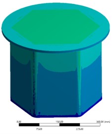
The following Fig.8 shows the Image of the water quality monitoring system. The monitoring system is composed of two parts. The upper device is filled with a batch of epe materials as the buoyancy supply material, and the shell is made of aluminum alloy, which can effectively resist the effects of ice layer temperature and expansion force. The lower device is the water quality monitoring instrument, with built-in sensors, batteries and other units for detection. It uses 3D printing resin materials. Upper and lower parts fixed by steel support, the water quality monitoring device is subject to the group standard T/CWEC13-2019 [10]. The water quality monitoring sensor is required to be 0.5 to 1.0 m underwater, the lower shell of the monitoring system is located between 0.4 m and 0.7 m under water, it can be seen from the above analysis that the ice thickness is one meter and the temperature rise rate is 10 ℃ /7200S.The external initial temperature is –20 ℃, analyze the temperature and equivalent stress of the monitoring System under the action of the ice layer temperature expansion force, as shown in Fig. 9, Fig. 10. It can be seen from the image that there is a stress concentration phenomenon at the edge of the water quality System.
To verify the accuracy of the numerical simulation, the extrusion experiment of ice thermal expansion force on the shell was carried out in the low-temperature environment simulation laboratory. The ice layer surface is heated by electric heating controlled the bottom water temperature is controlled by circulating heat exchange, and a miniature earth pressure sensor is pasted on the inner surface of the shell combined with a data acquisition instrument (DataTaker DT80) to form a data acquisition system. Control experimental conditions are consistent with simulation conditions. The maximum stress on the inner upper edge of the shell is 12.5 MPa, which is close to the simulation result, which verifies the accuracy of the numerical simulation. Although it is not far beyond the strength limit, However, ice attribute data for lower temperatures are lacking, and attention should also be paid here to engineering applications.
Fig. 8Image of the water quality monitoring system
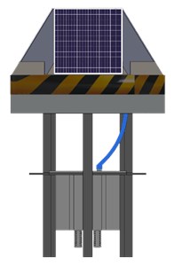
a) 3D structure image
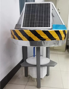
b) Physical image
Fig. 9Cloud chart of temperature
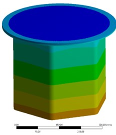
Fig. 10Cloud chart of equivalent stress
9. Conclusions
1) With the external temperature rise, the temperature field and stress field inside the ice layer show a non-linear distribution. It is not difficult to see that there is a one-to-one correspondence between the temperature field and the stress field by observing the distribution of the temperature field and stress field on the path. The temperature field is the smallest and the stress field is the largest.
2) With the increase of the external temperature rise rate, the thickness of the ice layer grows, the external initial temperature decreases, and the expansion force of the ice layer temperature shows an upward trend. The inflection point in the temperature and stress field is usually located at the upper 1/3 of the ice layer.
3) By calculating the structural response of the monitoring system in the ice layer, the simulation results show that there is a concentration of stress at the edge of the monitoring system, so there is a lack of ice material properties at lower temperatures, so the system will be more stressed under actual construction.
References
-
Li Jiting, “Research on the ice physical and mechanical parameters and ice surface bearing capacity of the Kanas Lake in the Xinjiang Uygur Autonmous Region,” Northeast Forestry University, 2017.
-
Zhang Sufeng, “Ice and interaction of bridge piers,” Northeast Forestry University, 2014.
-
Liu X. Z. et al., “Test and fracture toughness analysis for static ice pressure of reservoir slope,” Engineering Mechanics, Vol. 30, No. 5, pp. 112–117, 2013.
-
Shang Jian, “A study on ICE thermal expansive pressure action on large-scale pre-stressed aqueduct,” College of Water Conservancy and Hydroelectric, 2010.
-
Zhu Bofang, Thermal Stresses and temperature Control of Mass Concrete. Beijing: China Electric Power Press, 1999.
-
L. Fransson, “Thermal ice pressure on structures in ice covers,” Ph.D. Thesis, Lulea university of Technology, Sweden, 1988.
-
E. Kharik, B. Morse, V. Roubtsova, M. Fafard, A. Côté, and G. Comfort, “Numerical studies for a better understanding of static ice loads on dams,” Canadian Journal of Civil Engineering, Vol. 45, No. 1, pp. 18–29, Jan. 2018, https://doi.org/10.1139/cjce-2017-0142
-
Song Shuqing et al., “Research on thermal stress of cavity aqueduct,” China Rural Water and Hydropower, Vol. 11, pp. 86–88, 2005.
-
Liu Bo, “Finite element numerical solution of the thermal stress distribution in ice cover,” School of Civil Engineering, Tianjin University, 2004.
-
“Technical guidelines for spectral on-line water quality monitoring system,” China Water Resources Enterprise Association.
About this article

The authors would like to thank the national defense basic Scientific research program of China JCKY2019411B001, the Science and technology development plan project of Jilin province 20210201041GX, the Fund project of Jilin Provincial Department of Education No. JJKH20181124KJ.
The datasets generated during and/or analyzed during the current study are available from the corresponding author on reasonable request.
The authors declare that they have no conflict of interest.
