A multi-sensor cooperative detection target tracking method based on radar-optical linkage control

1. Introduction

Due to increased maneuvering characteristics, electronic countermeasures and the complexity of electromagnetic environment [1], there are many problems such as strong maneuvering characteristics, high filtering, multiple interference and increasing problems due to inefficiencies in checking [2]. Single target tracking is no longer able to adapt to the growing tracking requirements [3], which can result in incomplete measurements from optoelectronic tracking systems [4]. This results in wild and missing values in the sensor measurements, which increases the difficulty of estimating the target state in the information [5]. Based on this, this study aims to propose a multi-sensor co-detection target tracking method based on radar photoelectric linkage control. Firstly, based on radar photoelectric linkage control, the multi-sensor co-detection target tracking method is studied to carry out the construction of the mathematical model of the moving target. Then, an algorithm was selected for the multi sensor collaborative detection and target tracking method based on radar optoelectronic linkage control. Finally, the performance of the multi-sensor co-detection target tracking method is analyzed. Based on radar photoelectric linkage control, the multi-sensor co-detection target tracking method can solve the problems of unstable trajectory and large errors in the process of target tracking, which has strong relevance and research value. The innovation of this study lies in the construction of a mathematical model for moving targets based on a multi-sensor collaborative detection target tracking method using radar optoelectronic linkage control. In order to improve the target tracking performance of the mathematical model, an improved interactive multi-model (IMM) was proposed in the experiment based on traditional target tracking filtering algorithms and interactive multiple model algorithms. This algorithm enhances the radar detection and tracking effect and solves the problem of unstable track during target tracking.

2. Related works

In recent years, multi-sensor track fusion based on radar optoelectronic linkage control has been an important issue in multi-sensor tracking technology. Many scholars at home and abroad have done a lot of work and achieved rich results in multi-sensor research on track fusion in aircraft. Due to the requirements of anti interception and the limitation of the processing capacity of the fusion center, Zhang et al. [6] proposed an improved particle swarm optimization (MPSO) algorithm as a solution strategy for MIMO radars that perform target tracking and detection tasks. Extensive simulations verify that MPSO can provide performance comparable to that of the exhaustive search (ES) algorithm. In addition, MPSO has the advantage of simpler structure and lower computational complexity compared to multi-start local search algorithms. Dash and Jayaraman [7] introduced a sensor model based on a probabilistic approach for data fusion in multi-base radar. They observed that the probabilistic data fusion algorithm outperformed traditional data fusion algorithms. Man et al. [8] proposed a sensor-based method for dynamic radar echo simulation of targets by addressing the effect of radar sensors on radar echoes during measurements. And they analyzed the effect of sensors on radar echo simulation results. Na et al. [9] reconstructed the remaining radar echoes by interacting with “adjacent” sensor interactions to reconstruct the trajectory of the remaining targets. Distributed algorithms were used in the experiment as “descendants” of consensus protocols and random gradient descent. The numerical simulation illustrates the algorithm’s convergence. Li et al. [10] have developed an algorithm to solve the problem of linear arithmetic average (AA) fusion-based distributed multi-target detection and tracking problem. Two effective cardinality consensus methods for communication and computation were proposed in the experiment. They only propagate and fuse the probability of target existence between local MB filters. And simulation tests showed that the method is highly feasible in terms of accuracy, computational efficiency and communication cost.

Zhang and Hwang [11] proposed a multi-target identity management algorithm with two types of sensors. They combined it with existing multi-target tracking algorithms. And it finally demonstrated the effectiveness of the proposed algorithm through illustrative numerical examples. Cataldo et al. [12] introduced radar/telescope radio frequency systems for space surveillance and tracking applications related architecture, system and signal processing aspects, detailing its performance. Research has shown that programming technology and artificial intelligence also have good applications in target prediction [13]. In relevant literature, researchers have used computer programming technology, artificial intelligence, and other methods to predict the compressive strength of concrete. The results show that the hybrid model has high predictive performance and can be used for target prediction [14]. Zheng et al. [15] argued that multi-sensor Earth observation has significantly accelerated the development of multi-sensor collaborative remote sensing applications. And they proposed that the essential difference of depth models based on different sensor data training lies in the parameter distribution of sensor invariant and sensor invariant. Experimental results showed that deep multi-sensor learning outperformed other learning methods in terms of performance and stability.

In the above, it can be seen that there are many studies on sensor co-detection target. But there are few detection target tracking methods that combine radar photoelectric linkage control and multi-sensor co-detection target. For this reason, the research aims to innovate a multi-sensor co-detection target tracking method based on radar photoelectric linkage control. So it can enhance the radar detection tracking effect and solve the target tracking process such as track instability of target tracking.

3. Construction of a multi-sensor cooperative detection target tracking method based on radar-optical linkage control

3.1. Construction of a mathematical model of a moving target based on radar-optical linkage control of a multi-sensor cooperative detection target tracking method

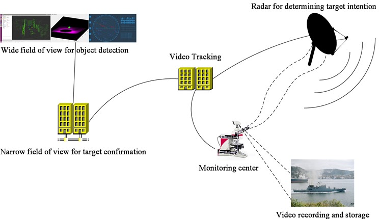
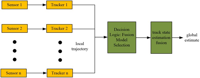
Currently, multiple radar joint detection systems are based on radar photoelectric linkage, with the monitoring area as the core and the mastery of the whole system. By locating and correcting the target, radar observes, identifies, and tracks the target, and searches and alarms the target within the monitoring range, and stores it on the local host. The operation should be configured with a working week scan or scan mode and operating range, and be able to set warning belts within the measurement area. The radar will continuously scan and report on the range [16]. As none of the environmental information perceived by humans is precise data, their decision-making process is mostly done with image thinking. While the photoelectric radar system understands the surrounding environment with precise data, the expressed use of image thinking is no longer able to complete the decision making. Once the radar detects the target, the target is detected. The target’s position, distance and velocity are translated into ground coordinates. Then the long-range optical camera and cameras will pinpoint the target. Based on the spectral method, the appropriate field of view and focus are derived by using the range and velocity parameters from the navigation information, respectively [17]. Firstly, a wide field of view is used to detect the object. Secondly, object recognition is achieved by zooming in on a narrow field of view. Ultimately, the image is tracked. And the travel path of the object, as determined by the radar, allows for further determination. When an alarm signal is displayed to a specified location, the monitoring system in the background starts recording and saves it. The radar detection and guidance control photoelectric tracking is shown in Fig. 1.

Fig. 1Schematic diagram of radar detection and guidance control electro-optical tracking (The ship photo was taken by authors)

Motion target tracking refers to the real-time tracking of moving objects. The moving state (speed, acceleration, etc.) of a manoeuvring object is an unpredictable and randomly changing characteristic. And the target moving pattern of current tracking systems deviates from the realistic moving state. So, the difficulty of estimating and forecasting its state is increased. To achieve effective tracking of targets, it is necessary to establish the target's movement mode reasonably and select appropriate filtering and tracking methods. In the case of manoeuvring target movements, it is difficult to be precise with an accurate numerical model due to the lack of sufficient a priori [18]. Therefore, there are only a few more accurate movement models for simulation under different conditions. In this study, the movement of a target is defined as a mere constant (CV) or one constant acceleration (CA) as a mathematical model. And the movement can be regarded as an arbitrary perturbation whose amplitude is reflected by a covariance matrix of the process. This method is the earliest and simplest method of tracking. Under continuous time conditions, CV mode refers to the uniform linear movement of an object. At point $t$, the state vector of the target is shown in Eq. (1):

1

$X\left(t\right)=\left[\begin{array}{c}x\left(t\right)\\ \dot{x}\left(t\right)\end{array}\right],$

where, $x\left(t\right)$ is the position of the target at moment $t$, $\dot{x}\left(t\right)$ is the velocity of the target at moment $t$ and $\ddot{x}\left(t\right)$ is the acceleration of the target at moment $t$. However, since the CV model only applies to targets travelling in a straight line at uniform speed, there is no acceleration, i.e. $\ddot{x}\left(t\right)=0$, as shown in Eq. (2):

2

$\ddot{x}\left(t\right)=w\left(t\right),$

where, $w\left(t\right)$ is the equation of state for the continuous period in which there is a random disturbance in velocity obeying a Gaussian distribution. Also known as the CV mode, it is described by Eq. (3):

3

$\dot{X}\left(t\right)=\left[\begin{array}{c}\dot{x}\left(t\right)\\ \ddot{x}\left(t\right)\end{array}\right]=\left[\begin{array}{cc}0& 1\\ 0& 0\end{array}\right]\left[\begin{array}{c}x\left(t\right)\\ \dot{x}\left(t\right)\end{array}\right]\text{+}\left[\begin{array}{c}0\\ \text{1}\end{array}\right]w\left(t\right).$

The CV model in continuous time is discretely varied to obtain the new CV model shown in Eq. (4):

4

$X\left(k+1\right)=\left[\begin{array}{ll}1& T\\ 0& 1\end{array}\right]X\left(k\right)+\left[\begin{array}{l}\frac{T^2}{2}\\ T\end{array}\right]w\left(k\right),$

where, $T$ is the sensor sampling period. In the time-continuous case, the CA model is described as a target in uniformly accelerated linear motion, and the state vector of the target at moment t is shown in Eq. (5):

5

$X\left(t\right)=\left[\begin{array}{c}x\left(t\right)\\ \dot{x}\left(t\right)\\ \ddot{x}\left(t\right)\end{array}\right],$

where, $x\left(t\right)$ is the position of the target at moment $t$, $\dot{x}\left(t\right)$ is the velocity of the target at moment $t$ and $\ddot{x}\left(t\right)$ is the acceleration of the target at moment $t$. In summary, the equation of state in continuous time, i.e. the CA model, is shown in Eq. (6):

6

$\dot{X}\left(t\right)=\left[\begin{array}{c}\dot{x}\left(t\right)\\ \ddot{x}\left(t\right)\\ \stackrel{⃛}{x}\left(t\right)\end{array}\right]=\left[\begin{array}{ccc}0& 1& 0\\ 0& 0& 1\\ 0& 0& 0\end{array}\right]\left[\begin{array}{c}x\left(t\right)\\ \dot{x}\left(t\right)\\ \ddot{x}\left(t\right)\end{array}\right]\text{+}\left[\begin{array}{c}0\\ 0\\ 1\end{array}\right]w\left(t\right).$

The CA model in continuous time is discretely varied. With a sampling period of $T$, the CA model is shown in Eq. (7):

7

$X\left(k+1\right)=\left[\begin{array}{lll}1& T& \frac{T^2}{2}\\ 0& 1& T\\ 0& 0& 1\end{array}\right]X\left(k\right)+\left[\begin{array}{l}\frac{T^3}{6}\\ \frac{T^2}{2}\\ T\end{array}\right]w\left(k\right).$

For linear movements with uniform linear velocity and uniform acceleration, both of the above modelling methods have good tracking results. However, if the target is maneuvering, that is, changing the acceleration vector of the target, applying the above methods will cause significant deviation. In this case, it is necessary to fully consider the maneuvering characteristics of the target and apply other modes, such as the current statistical model (CSM) mode described below [19]. The CSM model is essentially a model associated with a non-zero time. Its ‘current’ acceleration odds density is represented by a Rayleigh distribution curve, its plane average is the ‘current’ acceleration, and its stochastic acceleration is related to a time series. The CSM model is shown in Eq. (8):

8

$\left[\begin{array}{l}x\mathrm{\text{'}}\\ x\mathrm{\text{'}}\mathrm{\text{'}}\\ x\mathrm{\text{'}}\mathrm{\text{'}}\mathrm{\text{'}}\end{array}\right]=\left[\begin{array}{lll}0& 1& 0\\ 0& 0& 1\\ 0& 0& -\alpha \end{array}\right]\left[\begin{array}{l}x\\ x\mathrm{\text{'}}\\ x\mathrm{\text{'}}\mathrm{\text{'}}\end{array}\right]+\left[\begin{array}{l}0\\ 0\\ \alpha \end{array}\right]\stackrel{-}{a}\left(t\right)+\left[\begin{array}{l}0\\ 0\\ 1\end{array}\right]w\left(t\right),$

where, $\alpha$ is the correction parameter and $\stackrel{-}{a}\left(t\right)$ is the mean value of the correction parameter. The manoeuvring acceleration performance of the CSM model is expressed by a non-zero mean and a corrected Rayleigh distribution, which makes it more practical and more realistic. Based on this, the CSM model is used as the mathematical model for the motion target in this study.

4. Algorithm selection for a multi-sensor cooperative detection target tracking method based on radar-optical linkage control

The goal of filtering and forecasting is to estimate the moving state of a target based on its position, velocity, acceleration etc. In this thesis, the basic algorithm of IMM is chosen for an in-depth discussion. IMM is an interactive multi model algorithm that can adaptively adjust the probabilities of each model. At the same time, this algorithm can weight and fuse the state estimates of all models according to the corresponding probability to obtain a combined state estimate. Based on the pseudo-Bayesian interactive multi model algorithm, the corresponding model filters are designed according to different motion patterns by matching the motion patterns of multiple objects in multiple modes. The filter function of each action is separate and parallel. IMM can adjust the state of each mode appropriately based on different probabilities, thereby obtaining a comprehensive state evaluation [20]. It is assumed that IMM contains $n$ moving modes, where the discrete temporal state and observation equation for the $j$th moving mode $m_j$ is as follows:

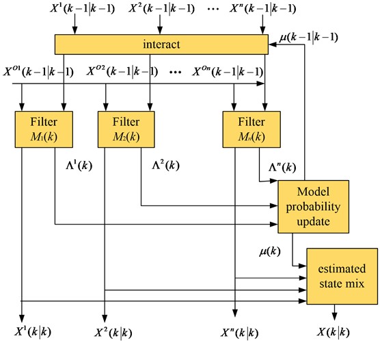
where, $X^j\left(k\right)$ represents the target state prediction matrix of the $k$ point-in-time movement model $j$, and $Z^j\left(k\right)$ represents the sensor measurements at $k$ time. $w\left(k\right)$, $\tilde{w}\left(k\right)$ represent mutually independent white noise. $G\left(k\right)$ represents the noise transfer matrix of the system, where the set of motion models of the system is $M=\{m_1,\cdots ,m_j,\cdots ,m_n\}$. The overall choice is to consider the full range of object motion conditions in an integrated manner. However, in practice, due to many constraints such as computational complexity and filter performance, the selection of $M$ should follow several basic guidelines. It is necessary to design with the smallest possible pattern. The interactive multi model consists of a filter, an inter-actor, an updater for model probability estimation, and a state estimation mixer that are suitable for various motion models. In Fig. 2 the process of constructing the n operational models for the IMM algorithm is shown.

Fig. 2The flow chart of the structure of the IMM algorithm

In the IMM algorithm, the following guidelines must be followed when selecting the target motion mode. It needs to cover the most real targets with the smallest motion mode. Therefore, when using the IMM method for target tracking, a larger number of models needs to be selected to achieve better tracking results. However, if the model number is too large, this can lead to increased differences between the different models and more transitions. This can lead to inappropriate matching between models, resulting in state estimation errors and even filtering divergence in the IMM algorithm. The problem of model mismatch exists in IMM algorithms that introduce both CV and CA models. The reasons for the model mismatch are analyzed below and improvements to the corresponding algorithms are given. The method still uses two measurements as initial filters under the CA model. But a state variable is added to the prediction of the CA model, thus compensating for the larger errors due to the model mismatch. After the initial trajectory, a position vector of the target including factors such as position and velocity is obtained by the target tracker. That is, the initial values and initial covariance of each motion model have been obtained in the IMM algorithm, as shown in Eq. (10):

where, $\widehat{X}\left(1\left|1\right.\right)$ denotes the initial state and contains the error value, $\widehat{P}\left(1\left|1\right.\right)$ denotes the initial covariance and contains the error value. In the 3D Cartesian coordinate system, for the CV model, in order to match the CA model matrix dimension, the dimension of the state transition matrix of the CV model is 9×9. The state transfer matrix of the CV model is shown in Eq. (11) and (12):

In each recursive loop of the IMM algorithm, this improved IMM algorithm takes known data from the previous time and adds the acceleration term to the CA model to compensate for the current situation. By fusing the IMM inputs, the mismatch challenge between the CA and CV models can be well overcome. So the tracking stability of the IMM algorithm is improved. And the trajectory at the current time is obtained by filtering the existing point in time correction. Structural fusion can be performed based on two different flight paths. These two types of trajectories are the fusion of sensor trajectories and sensor motion trajectories, as well as the combination structure of sensor trajectories and sensor trajectories based on system trajectories. The fusion structure of the sensor trajectory and the sensor track is shown in Fig. 3.

Fig. 3Fusion structure diagram of sensor track and sensor track

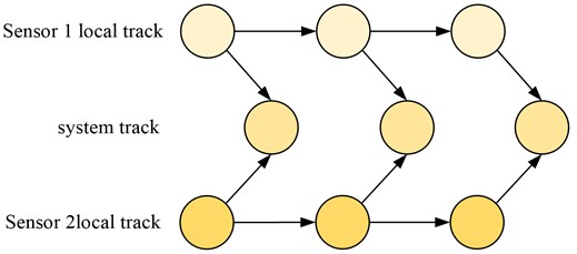
In the combined diagram of the two different types of sensor trajectories, the trajectories of the upper and lower two different types of sensors are used, while two different paths are used at the fusion centre. The timings in the chart are arranged sequentially from left to right. At the fusion centre, multiple sensors are fused simultaneously to obtain the new trajectory. Due to this method of fusion, the trajectories at each point in time are independent of each other and there are no errors in correlation estimation. This means that correlation and trajectory estimation errors are not propagated over time. Although this fusion method is simple and easy to implement, its performance is not sensitive enough. The track fusion structure of the sensor tracks and the system tracks is shown in Fig. 4.

Fig. 4Fusion structure diagram of sensor track and system track

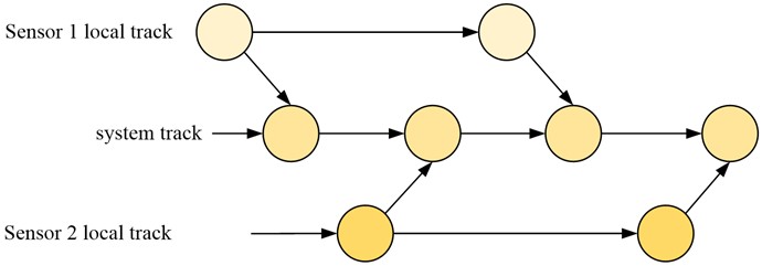
In the fusion of the tracks of the sensors and the system, the sequence is generated by random from right to left. If a new detection track appears at the present time, the target is tracked by the method in that area. By matching and fusing with the trajectory of the sensor, the estimated route state of the system at that time point was ultimately obtained, thus forming the trajectory of the system. The current timing was used as previous estimates of the system state in the fusion. As previous correlation and merging errors can have an impact on the fusion results, a correlation algorithm is used to remove the errors. In complex electromagnetic backgrounds, the fusion effect of simple and easy to implement algorithms is poor. Therefore, it is necessary to adopt algorithms with good characteristics, but their structure is complex and computational complexity is large. In order to meet the need for good performance and computation, the fusion of track information from multiple sensors can be widely used in various environments. Based on this, this research applies the adaptive track fusion method, and the adaptive track fusion structure is shown in Fig. 5.

Fig. 5Adaptive track fusion structure diagram

The principle of adaptive trajectory fusion algorithm is as follows: n received measurements were tracked and filtered, and the trajectories of each target were obtained and fused. The core of this fusion consists of two main elements, namely judgemental reasoning and trajectory integration. The paths are fused based on certain criteria, and the paths are integrated and evaluated by selecting a suitable fusion method. A multi model fusion decision tree is constructed based on the fusion algorithm of decision statistical spacing and decision tree, as shown in Fig. 6.

Fig. 6Multi-model fusion decision tree

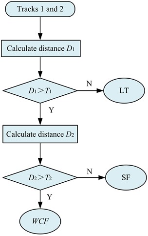
A multi-modal fusion decision tree based on the steps comprising. Firstly, it needs find the maximum distance D1, based on the input target trajectory. When D1 is lower than the threshold T1, it means that the positions between the two targets are very similar. So the decision tree estimates the position of local track (LT) as a whole. If the distance D1 is larger than the threshold T1, then the second statistical distance D2 is found. If D2 is lower than the threshold T2, it means that the mutual covariance between the sensor trajectories is very small and can be disregarded. On this basis, a least squares-based decision tree was used for the integrated state estimation. In the case that D2 is larger than the threshold T2, the covariance term of the tracking deviation of each sensor cannot be neglected. Therefore, a fusion method based on the covariance values was used on the decision tree for the overall state estimation. The first statistical spacing D1 is the spacing between the sensor trajectory and the system track state estimate obtained by the simple fusion (SF) algorithm, which is calculated as shown in Eq. (13):

where, ${\widehat{x}}_1$ is the state estimate of sensor 1, ${\widehat{x}}_{SF}$ is the coefficient of fusion status of the SF algorithm for estimating sensors 1 and 2, $p_{SF}$ is the covariance of the fusion deviation of sensors 1 and 2 based on the SF approach, and $p_1$ is the error covariance of sensor 1. The second statistical spacing D2 is the distance between the sensor trajectory and the state estimate of the WCF algorithm-based system, as shown in Eq. (14):

where, ${\widehat{x}}_{WCF}$ is the fusion state estimate of sensors 1 and 2 based on the weighted covariance fusion (WCF) algorithm. And $p_{WCF}$ is the fusion error covariance of 1 and 2 based on WCF. The adaptive track fusion algorithm based on system performance requirements can dynamically select suitable fusion algorithms, thereby improving computational efficiency and fusion effect while fully considering computational complexity. Moreover, this method can adjust the accuracy of fusion based on changes in threshold. In order to verify the stability and reliability of the model in practice, this study uses RMSE as the evaluation index, as shown in Eq. (15):

where, $n$ is the total number of samples. $\tilde{Y}$ is the predicted value of the $i$th sequence. $Y\left(i\right)$ is the actual value of the $i$th sequence.

5. Performance analysis of a multi-sensor cooperative detection target tracking method based on radar-optical linkage control

First, in order to verify the basic performance of the algorithm proposed in the study, compare the effect of IMM algorithm in basic database training. Nuscence is used as the training data set in the study. The data set has 1000 scenes, including multiple scenes such as roads and infrastructure. Each scene has a length of 20 s and 2 key-frames per second. The improved IMM algorithm is trained and learned. And the average error of the algorithm and the traditional IMM algorithm is evaluated in the $X$ and $Y$ directions, as shown in Fig. 7.

Fig. 7(a) shows the comparison results of error calculation differences between the traditional IMM algorithm and the improved IMM algorithm in $X$ direction. It can be seen that the error value of the improved IMM algorithm changes slightly with time, while the error value of the traditional IMM algorithm changes significantly. Fig. 7(b) shows the comparison results of the error differences between the two algorithms in $Y$ direction. It can be found that, as time increases, the error value of the improved IMM algorithm does not exceed 20 m. While the error value of the traditional IMM algorithm exceeds 20 m at multiple time points. The above results show that the improvement of IMM algorithm is effective. Its error value is smaller than the traditional IMM algorithm, and it has higher accuracy in target tracking.

Fig. 7Position error of improved IMM algorithm

a)$X$ direction

b)$Y$ direction

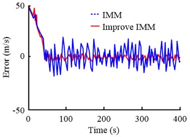
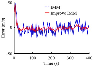
Secondly, in order to analyze the stability of the proposed method in the calculation process, the speed errors of different algorithms are compared in the target tracking process, as shown in Fig. 8.

Fig. 8Speed error of improved IMM algorithm

a)$X$ direction

b)$Y$ direction

It can be seen from Fig. 8 that the stability of the target tracking process is evaluated by calculating the speed error of the improved IMM algorithm. It can be found that the tracking speed of the IMM algorithm used in the study does not change significantly. And compared with the traditional IMM algorithm, its speed error continues to remain at 0 m/s. The above results show that, in the long tracking process, the speed of the improved IMM algorithm can always maintain a relatively stable state. That is, it can achieve real-time target tracking.

Fig. 9The target is doing a uniform linear motion trajectory

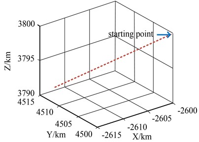
Through Matlab simulation and standard simulation, the effectiveness of this method in practical application is compared IMM algorithm. In the simulations, the number of Monte Carlo was 1000 and the initial model probability was set to $\mu =\text{[0.25, 0.25, 0.25}\text{, 0.25]}$ for a sampling time of 0.2 seconds. It is assumed that the target starting position is (–2610 km, 4510 km, 3810 km) and the starting velocity is set to (–220 m/s, 225 m/s, 165 m/s) in a 3D right-angle coordinate system. And the target which makes a uniform linear motion with the trajectory is shown in Fig. 9.

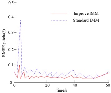
As can be seen in Fig. 9, the target is making uniform linear motion. But the differences and performance between the standard IMM algorithm and the improved IMM algorithm need to be investigated for further validation. So the study will do further analysis of the target’s orientation and pitch tracking errors based on both algorithms, as shown in Fig. 10.

Fig. 10Comparison of standard IMM and improved IMM algorithm

a) Azimuth error map

b) Pitch error map

As shown in Fig. 10, the tracking error of the standard IMM algorithm was analyzed in terms of heading and longitudinal tilt tracking error. It was found that the tracking error curve of the standard IMM fluctuated less in the absence of other movement patterns. The tracking accuracy and attitude tracking accuracy of the system were less than 0.2 degrees. As the object is a straight line, its movement pattern is constant. Therefore, there is no model mismatch in the conversion of motion patterns, such as CV, CA. Assuming that in the 3D Cartesian coordinate system, the starting position of the object is (–2610 km, 4510 km, 3810 km) and the initial velocity is (–220 m/s, 225 m/s, 165 m/s). The movement of the object is as follows: 0 to 15 seconds is a straight line. 15 to 30 seconds is a movement to the left with an angular velocity of 0.069 rad/s. 30 to 45 seconds is a right turn movement with an angular velocity of –0.06931 rad/s. 45 to 60 seconds is a uniform straight line with an acceleration of 5.6846 m/s. The trajectory of the target is shown in Fig. 11.

Fig. 11The target is doing a variable speed trajectory

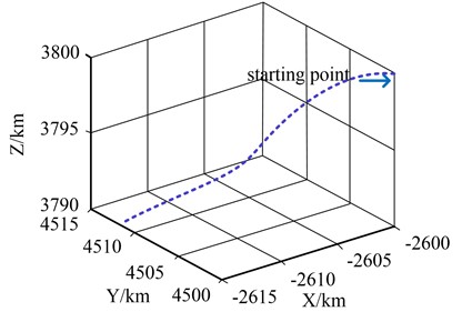
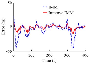
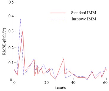
From Fig. 11, it can be seen that the target is doing variable speed motion. But the difference and performance between the standard IMM algorithm and the improved IMM algorithm are different from target characteristics when it is in uniform linear motion. So the study will do an analysis of the target’s orientation and pitch tracking error based on the two algorithms when the target is doing variable speed motion. The analysis effect is shown in Fig. 12.

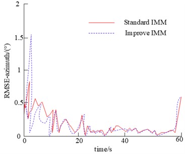
Fig. 12Comparison of standard IMM and improved IMM algorithm

As can be seen from the heading and aspect tracking error plots, the traditional IMM method has a large variation in the heading and aspect tracking error curves. There are significant changes in the switching between CV and CA modes. The highest values of error are between 15 and 30 seconds, 30 and 45 seconds, and 45 and 60 seconds. It indicates the problem of model mismatch when switching between motion modes such as CV and CA for the standard IMM algorithm. Due to the transition of the motion modes from CV to CA, the state parameter acceleration from none to none is necessary. It results in a gradual increase in bearing and pitch tracking errors, which are within 0.2° of the heading and pitch tracking errors relative to the conventional IMM algorithm. The results show that the method can well solve the model mismatch problem of CV and CA motion modes at the transition.

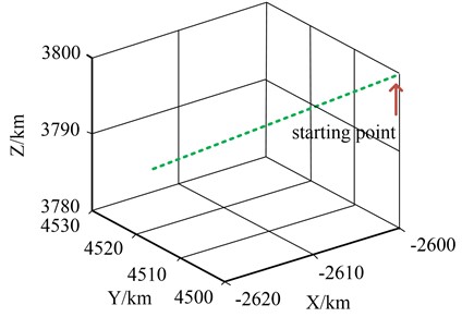
Using a simple trajectory fusion method that allows tracking of multiple sensors as well as a single sensor, simulations of single-sensor electronic support measures (ESM), ESM, multi-sensor ESM, and infrared search and track (IRST) are investigated. Among them, ESM is electronic reconnaissance, which can search, intercept, locate, record, and analyze radiated electromagnetic energy. IRST is a measurement system using infrared as the medium. Based on this, iterative updates were performed using adaptive filters to obtain information on the position and velocity of the target. In the simulations, the Monte Carlo count was 100, the sampling time was 1 s and the object made a uniform linear motion, the trajectory of which is shown in Fig. 13.

Fig. 13The target is doing a variable speed trajectory

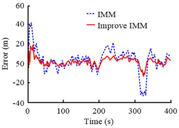
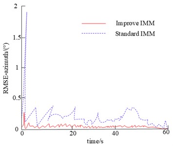
The orientation tracking error, pitch tracking error for single sensor ESM, multi-sensor ESM and IRST are shown in Fig. 14.

In terms of comparative orientation and pitch tracking for single sensor ESM, multi-sensor ESM and IRST, the tracking error for both methods is less than 0.1 degrees. However, the tracking error for multiple sensors is lower, the curve undulates more smoothly and has a higher stability. From this, it can be seen that better tracking results can be obtained by using multiple sensors for track fusion after the introduction of IRST with high accuracy.

Fig. 14Single-sensor and multi-sensor error comparison chart

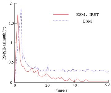
a) Azimuth error map

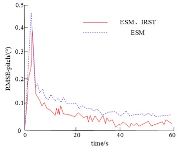
b) Pitch error map

6. Conclusions

Radar can be used for observing, identifying, and tracking targets, and for searching and alerting targets within the monitoring range [16]. Meanwhile, research has shown that using optoelectronic devices and parameters such as distance measurement and velocity measurement in navigation data can determine appropriate field of view and focus for target tracking. Currently, some studies have combined radar with optoelectronic devices to achieve linkage control [21]. The target tracking and photography technology based on radar optoelectronic linkage control mainly monitors dynamic targets in the monitoring area. It achieves the goal of radar grasping the overall situation and precise photography by optoelectronic devices. However, the current technology has problems such as poor detection and tracking performance, and unstable trajectory during target tracking [22]. Therefore, the research aims to innovate a multi-sensor collaborative detection target tracking method based on radar optoelectronic linkage control, and construct a mathematical model of moving targets. In order to improve the target tracking performance of the mathematical model, an improved IMM algorithm was proposed in the experiment based on traditional target tracking filtering algorithms and interactive multiple model algorithms. In the simulation experiment, the results showed that the improved IMM algorithm had heading and pitch tracking errors within 0.2° for the target in variable speed motion. This algorithm can effectively solve the problem of model mismatch during the conversion of motion modes such as CV and CA. Moreover, the tracking error of multiple sensors is low, and the curve undulation is relatively smooth, with high stability. After introducing high-precision IRST, using multiple sensors for track fusion can achieve better tracking results. The results confirm that the improved algorithm enhances the radar detection and tracking effect, and solves the problem of unstable track during target tracking.