Abstract
This study develops an empirical model to predict the airflow resistivity of thin and low-density sound-absorbing materials. Airflow resistivity is a key input parameter for Finite Element Method (FEM) simulations of sound pressure levels (SPLs) in vehicle cabins. However, existing models for determining the airflow resistivity of thin and low-density fibrous materials are inaccurate. Therefore, this study proposes a simple and reliable model based on multiple linear regression analysis of polypropylene fibrous nonwoven samples. The samples were tested using equipment designed according to ISO standards 9053-1. The model selection was performed using stepwise techniques to identify the most relevant predictors. The final model, along with its coefficients and goodness of fit statistics, is presented and discussed. The results of this study offer a practical tool for design engineers to estimate the airflow resistivity of thin and low-density materials, which can improve the accuracy of FEM simulations of SPLs in vehicle cabins.
Highlights
- The current airflow resistivity models are not flexible and are limited to a specific thickness and density range.
- Currently, there are no empirical models that can accurately predict the airflow resistivity of thin, low-density sound-absorbing materials.
- An empirical model that can accurately predict the airflow resistivity of thin, low-density sound-absorbing materials was successfully developed in this work using multivariable regression analysis.
1. Introduction
The Finite Element Method (FEM) allows designers to model a product in a virtual environment, eliminating the need for physical prototypes early in the design phase. When developing and testing a new vehicle prototype, noise, and vibration engineers use FEM models to determine the effect sound-damping material have on internal noise levels. Therefore, accurate sound absorption models are important for predicting sound pressure levels (SPLs) in the vehicle cabin. FEA software packages such as COMSOL Multiphysics, ANSYS Acoustics, and Actran require airflow resistivity as an input parameter for predicting sound propagation and absorption in porous materials. These software packages enable modelling of sound waves interacting with porous materials, and the airflow resistivity is a key material property that affects the sound absorption behaviour of these materials.
The development of numerous empirical models for predicting airflow resistivity of fibrous materials has been seen in recent years, with a focus on naturally occurring materials. Research published by Dunne et al. [1], discussed the available models and their working range in great detail, covering a broad range of bulk densities and fibre diameters. The models are reported to be valid over the bulk density range of 12-132 kg/m3 and fibre diameter range of 11-75 μm. The accuracy of the models were benchmarked against real-world data, showing that the Modified Ballagh model performed well on synthetic fibres but poorly on natural fibres, while the Bies model performed best on natural fibres. It was found that the models are not very flexible and are limited to a specific range, with poor predictions for thin low-density fibrous sound absorbing materials. This presents a challenge for design engineers who use predictive models to determine the airflow resistivity of thin, low-density materials.
Thus, this research develops a novel airflow resistivity model that can accurately predict the airflow resistivity of thin ( 20 mm), low-density ( 50 kg/m3) materials.
2. Material development
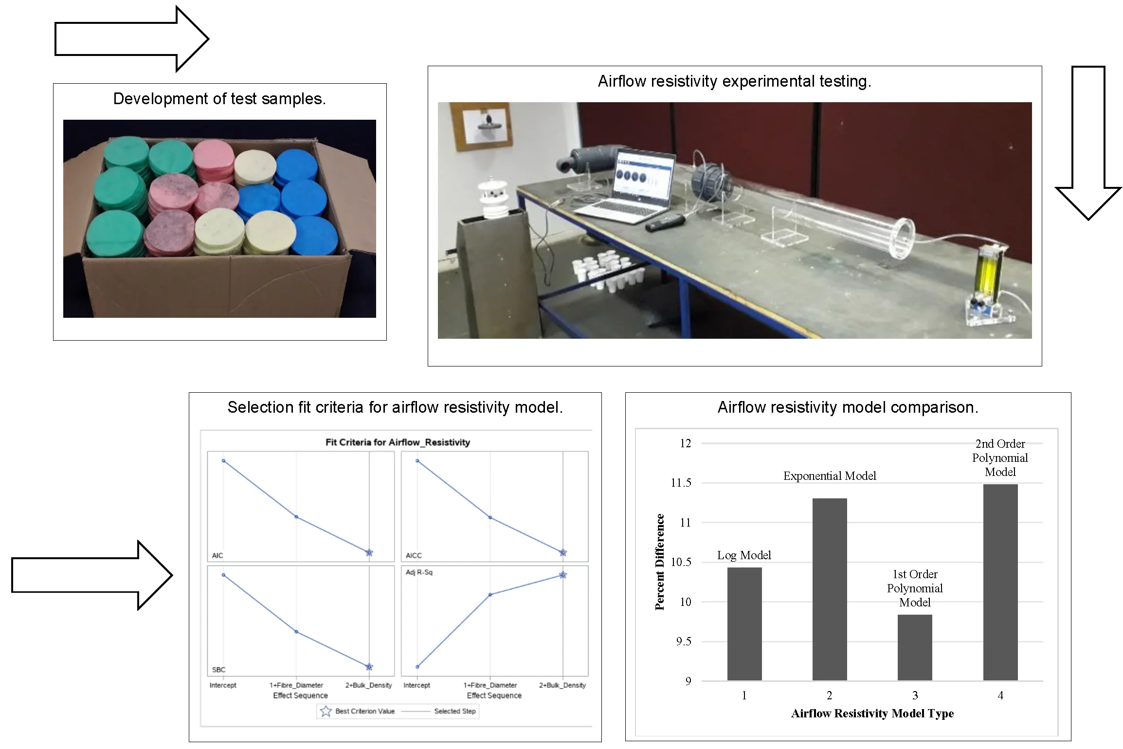
The research used equipment designed according to ISO standards 9053-1, with the experimental equipment manufactured to high-quality specifications. The airflow resistivity tube was used to test the airflow resistance of different polypropylene fibres of varying diameters that were manufactured into nonwovens, illustrated in Fig. 1. A total of 203 samples were used, with 180 used for model development and 23 for model validation. The thickness, bulk density, and airflow resistivity of each sample were measured using calibrated equipment. The experimental setup for the airflow resistivity testing involved preparing the laboratory environment, randomizing the order of testing, and using calibrated equipment, including a testo 512 pressure meter (0- 200 Pa), with a resolution of 0.1 Pa, KOFLOC flow meter model RK120X series capable of measuring flows as low as 5 ml/min, and a MaxiMet (GMX501) Compact Weather Station. Note, due to the large amount of data captured for this study only summarised tables are given as seen in Table 1 and 2.
Fig. 1Airflow resistivity experimental setup taken in September 2022 by RK Dunne in the sound and vibration lab at TUT
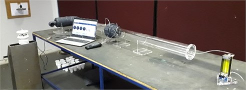
Table 1Model development dataset
Sample No. | Thickness (mm) | Bulk density (kg/m3) | Airflow resistivity (Pa.s/m2) | Fibre diameter (μm) |
Average | 10.61 | 35.62 | 6936.49 | 35.20 |
Minimum | 7.0 | 20.32 | 1023.34 | 19.40 |
Maximum | 15.20 | 50.76 | 23843.63 | 49.50 |
Table 2Model validation dataset
Sample No. | Thickness (mm) | Bulk density (kg/m3) | Airflow resistivity (Pa.s/m2) | Fibre diameter (μm) |
Average | 10.80 | 39.51 | 6412.99 | 35.20 |
Minimum | 6.90 | 21.89 | 2871.38 | 19.40 |
Maximum | 17.0 | 53.39 | 11865.01 | 49.50 |
3. Parameter analysis and selection
Regression models show the mathematical relationship between a predictor variable and a response variable. When no theoretical knowledge of the relationship is available, the choice of the model is based on an inspection of scatter plots. In this study the method of least-squares is used to develop the empirical airflow resistivity model. Furthermore, multiple linear regression is used since the model contains more than one independent variable.
Linear models assume the mean of is linearly related to , the error terms are normally distributed with a mean of zero and equal variances, and the error terms are independent at each value of the predictor variable. Model development involves an iterative process of selecting regressor variables and identifying the best equation to fit the data. ANOVA, R-squared, and information criteria were used to aid in evaluating the quality of the relationship between the response and predictor variables.
3.1. Collinearity check
Collinearity can cause instability in a model and must be checked for and removed. The airflow resistivity data were analyzed using SAS software and the Variance Inflation Factor (VIF) was calculated, with a cutoff value set at 10. Mass, thickness, bulk density, and porosity had VIF values greater than 10, indicating collinearity. After removing mass and porosity, the VIF dropped to acceptable levels, indicating significant collinearity between these predictors and the others. The redundancy of these predictors will be further illustrated in subsequent sections.
3.2. Model selection
The process of selecting candidate models involves evaluating and selecting models based on various criteria. These criteria include significance levels (-values), information criteria (such as AIC, AICC, BIC, and SBC), and adjusted R-squared values.
To illustrate the process of selecting candidate models, the example of selecting the best predictor variables for airflow resistivity is used. With five possible predictors, there are 32 possible models, so it is necessary to eliminate the least significant predictors. This can be done using stepwise model selection techniques such as forward selection, backward selection, and stepwise selection.
The SAS software is used to perform the model selection process. The STEPWISE model selection technique is implemented to select the most appropriate subset of models. The process starts with all the variables in the dataset and eliminates the least significant variables based on a significance level of 0.05.
The SAS output displays tables and graphs that provide information about the model selection process at each step. The Coefficient Progression for Airflow Resistivity shows how the standardized coefficients and the criterion were used to choose the final model. The set of fit criteria, AIC, SBC, AICC, and adjusted R-squared values for each step are plotted and compared side-by-side as seen in Fig. 2.
Fig. 2Selection fit criteria for airflow resistivity model
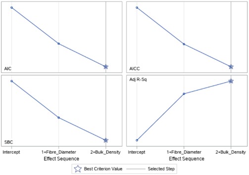
The stepwise process based on significance level chose the model at Step 2, which includes both fibre diameter and bulk density. This model produced the lowest Average Squared Error (ASE) value, indicating less unexplained variation in the Airflow Resistivity model. As can be seen, the mass and porosity parameters were illuminated thus confirming the collinearity analysis.
Beyond significance levels, information criteria can also be used to evaluate and select models. Each criterion searches for a model that minimizes unexplained variability using as few effects as possible. These criteria are helpful in directing the selection process within the SAS software procedure.
In summary, selecting candidate models involves evaluating and selecting models based on various criteria such as significance levels, information criteria, and adjusted R-squared values. The SAS software is a useful tool for performing the model selection process and provides tables and graphs to help interpret the results.
4. Regression model development
Upon analysis of the airflow resistivity data scatter plots, a non-linear relationship with the fibre diameter was found, so a transformation was applied to the data to enable linear regression analysis. However, the choice of model for the transformed data is not straightforward. Different models, such as logarithmic, exponential, power, or polynomial models of varying orders, could all potentially fit the data well. Therefore, a model selection process is necessary to determine the best model for the available data.
4.1. Model comparison
The model selection process requires applying the data to each model and analysing which model gives the highest adjusted R-squared value. During this process, numerous possible combinations of the variables were checked to see which combination would give the highest adjusted R-squared value for the dataset, the data analysis tool in Microsoft Excel was utilized to perform this. The result of this process is expressed in Table 3.
It is evident from Table 3 that the Log-Log model gave the highest adjusted R-squared value. At this point in the research, it is still too early to select the best model since other factors must be brought into the selection process. The additional factors, the selection of the best model and its mathematical derivation will be discussed in the coming sections.
Table 3Airflow resistivity model R-squared comparison
Combinations | Fibre diameter/bulk density () | Fibre diameter () | Bulk density () |
Model type | |||
Log-Log | 0.966 | 0.744 | 0.202 |
Exponential | 0.949 | 0.735 | 0.199 |
First-order polynomial with one-interactions | 0.867 | – | – |
Second-order polynomial with one-interactions | 0.952 | – | – |
5. Final model selection and validation
In order to select the most accurate model for future predictions, it is necessary to test the models on a validation dataset. Then, the performance of the models must be compared to determine which one performs the best. Additionally, the selected model must be checked to ensure that it meets the assumptions required by linear regression, such as a linear relationship between the predictor and response variables, normally distributed error terms with a mean of zero, equal variances, and independent error terms at each value of the predictor variable.
5.1. Airflow resistivity model selection
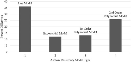
The validation dataset was used to assess the developed airflow resistivity models, and it was found that the 1st order polynomial model had the lowest average percentage difference between the measured value and the predicted value. The models were also evaluated against an external dataset, and a selection metric was developed to objectively select the best model. The Exponential model outperformed all competing models on the external datasets and had the highest average selection metric score and thus was chosen as the best model. Figs. 3 and 4, show the percentage difference between the actual and predicted airflow resistivity values predicted by each model. It should be noted that the external dataset was made up of both synthetic fibres and natural fibres.
Fig. 3Airflow resistivity model comparison using validation dataset
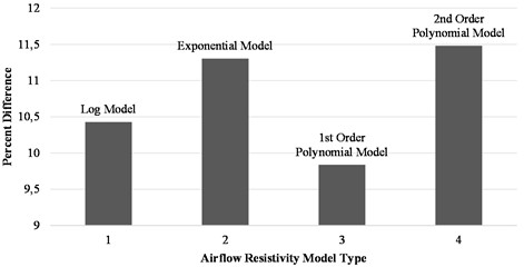
Fig. 4Airflow resistivity model comparison using external dataset
5.2. Validating model assumptions
The assumptions of the model, including linearity, independence, normality, and homogeneity of variances, were validated before using the model for future predictions. The influential observations were also tested using the software NumXL [2], and no adjustments were necessary. Model linearity was validated using scatter plots, while normality assumptions were validated using a histogram plot of the residuals. The independence and equal variance assumptions were validated using a residual plot of the errors.
5.3. Model derivation
Linear regression analysis was used to develop the airflow resistivity model, which was benchmarked against existing models to evaluate its performance. The non-linear behavior observed in the airflow resistivity data required data transformation for linear regression. The regression analysis showed that only fibre diameter and bulk density are significant predictors of airflow resistivity. The adjusted coefficient of determination value obtained for the Exponential model was 0.949, indicating that 94.9 % of the variability in the data is explained by the model. The resulting equation is expressed in non-linear form in Equation 1, with airflow resistivity as a function of fibre diameter and bulk density:
where is the airflow resistivity in Pa.s/m2, is the fibre diameter in μm, and is the bulk density in kg/m3.
5.4. Airflow resistivity model comparison
The developed airflow resistivity model was compared against twenty-five existing models. Table 4, shows the data for the best performing modes. The average, minimum and maximum percentage difference between the actual and predicted airflow resistivity of these models is compared with the developed Exponential model in Table 4.
The external data used to produce Table 4, was obtained from the following references; [7], Li et al. [8], and Yang et al. [9]. As it can be seen from Table 4, the current models lack prediction consistency with high variation between the predicted minimum and maximum percentage differences.
Table 4Performance of current airflow resistivity models
Model performance | %Diff external data | %Diff internal data | Ref |
Kozeny-Carman | Avg: 57.33 Min: 10.92 Max: 142.07 | Avg: 16.04 Min: 0.24 Max: 38.34 | [3] |
Ballagh | Avg: 42.36 Min: 0.62 Max: 59.53 | Avg: 24.16 Min: 1.70 Max: 65.72 | [4] |
Sullivan | Avg: 37.16 Min: 5.01 Max: 109.04 | Avg: 13.11 Min: 2.85 Max: 31.21 | [5] |
Yilmaz | Avg: 47.84 Min: 0.36 Max: 139.69 | Avg: 59.46 Min: 0.24 Max: 181.99 | [6] |
Developed exponential model | Avg: 12.10 Min: 3.55 Max: 27.05 | Avg: 11.35 Min: 0.061 Max: 25.66 |
6. Conclusions
This study aimed to address inaccurate predictions of sound pressure levels within vehicle cabins when using FEA software. The current FEA software utilizes empirical models that are not developed for thin, low-density materials. By testing multiple models, it was found that the Exponential model accurately predicted airflow resistivity, demonstrating flexibility and accurate predictions of both synthetic and natural fibres of different bulk densities and thicknesses. Although the developed model performs well caution should be exercised when applying this model to data outside of its developed range since empirical models are only accurate within a specified range they were developed for.
References
-
R. K. Dunne, D. A. Desai, and P. S. Heyns, “Development of an acoustic material property database and universal airflow resistivity model,” Applied Acoustics, Vol. 173, p. 107730, Feb. 2021, https://doi.org/10.1016/j.apacoust.2020.107730
-
“NumXL. NumXL – Analytics Made Easy!,” https://numxl.com/, 2022.
-
M. T. Pelegrinis, K. V. Horoshenkov, and A. Burnett, “An application of Kozeny-Carman flow resistivity model to predict the acoustical properties of polyester fibre,” Applied Acoustics, Vol. 101, pp. 1–4, Jan. 2016, https://doi.org/10.1016/j.apacoust.2015.07.019
-
N. D. Yilmaz, “Acoustic properties of biodegradable nonwovens,” in Textile Technology Management, 2009.
-
F. P. Mechel, Formulas of Acoustics. Springer, 2002.
-
N. Yilmaz et al., “Effects of porosity, fiber size, and layering sequence on sound absorption performance of needle-punched nonwovens,” Journal of Applied Polymer Science, Vol. 121, pp. 3056–3069, 2011.
-
M. Garai and F. Pompoli, “A simple empirical model of polyester fibre materials for acoustical applications,” Applied Acoustics, Vol. 66, No. 12, pp. 1383–1398, Dec. 2005, https://doi.org/10.1016/j.apacoust.2005.04.008
-
C. D. Li et al., “Material parameter determination in glass wool mat for sound absorption,” Applied Mechanics and Materials, Vol. 148-149, pp. 1271–1275, Dec. 2011, https://doi.org/10.4028/www.scientific.net/amm.148-149.1271
-
T. Yang et al., “Study on the sound absorption behavior of multi-component polyester nonwovens: experimental and numerical methods,” Textile Research Journal, Vol. 89, No. 16, pp. 3342–3361, 2018.
About this article

The authors have not disclosed any funding.
The datasets generated during and/or analyzed during the current study are available from the corresponding author on reasonable request.
The authors declare that they have no conflict of interest.
