Prediction and evaluation of polymer turbulent drag reduction efficiency based on BP neural network

Chen, Yang; He, Minglan; Zhang, Meiyu; Luo, Jin

doi:10.21595/lger.2023.23661

Liquid and Gaseous Energy Resources

Browse Journal

Submit article

Published: 30 October 2023

Check for updates

Prediction and evaluation of polymer turbulent drag reduction efficiency based on BP neural network

Yang Chen¹

Minglan He²

Meiyu Zhang³

Jin Luo⁴

¹Institution of Oil-Gas Storage and Transportation, Ufa State Petroleum Technological University, Ufa 450062, Russia

^{1, 2, 3, 4}Petroleum Engineering School, Southwest Petroleum University, Chengdu, 610500, China

^{2, 3, 4, 1}National Key Laboratory of Oil and Gas Reservoir Geology and Exploitation, Southwest Petroleum University, Chengdu, 610500, China

Corresponding Author:

Yang Chen

Cite the article Download PDF

Downloads 84

Abstract

In the process of oil exploitation and transportation, in order to effectively predict and control energy consumption for drag reduction of oil flow, in this paper a BP neural network was proposed based method for predicting and evaluating the turbulent drag reduction efficiency of polymers, which can greatly improve the current situation of relying on empirical formulas and low generality in polymer turbulent drag reduction efficiency prediction. Based on the experimental data sets of four commercial polymer drag-reducing agents FLOXL, М-Flowtreat, Necadd-447, and FLO MXA, obtained at different polymer concentrations, viscosity, density, and Reynolds number, a BP neural network has been established and the optimal number of neurons in the hidden layer was selected using the root mean square error (RMSE) value to obtain the optimal BP neural network prediction model. The BP neural network prediction models for the four polymer drag-reducing agents all have a good fit of 0.98 or above, and the $R^{2}$ of the trained BP neural network for the Necadd-447 drag-reducing agents is 0.9949, which is the best among the four polymer drag-reducing agents. The BP neural network established in this paper can be applied to the turbulent drag reduction transport of long-distance pipelines for oil products to achieve the prediction of the drag reduction efficiency of polymer additives.

Prediction and evaluation of polymer turbulent drag reduction efficiency based on BP neural network

Highlights

A BP neural network-based approach is proposed to predict the turbulence drag reduction efficiency of polymers, which can reduce the reliance on empirical formulas and improve the accuracy and applicability.
By applying the experimental dataset, comparing the RMSE values, selecting the optimal number of neurons in the hidden layer, 10-fold cross-validation has been utilized to ensure the reliability and generalization of the model.
The prediction of drag reduction efficiency of polymer additives in long-distance pipelines has been achieved by the proposed BP neural network.

1. Introduction

In the process of long-distance pipeline transport of refined oil products, the flow at a high Reynolds number will produce huge turbulence loss, very low concentration (one millionth) of polymer drag reducer can significantly reduce turbulence loss and improve pipeline transport capacity, so the polymer drag reducer is widely used in long-distance pipeline transport of refined oil products [1].

At present, there are many types of polymers used in oil pipeline transport, the polymer drag reduction efficiency is closely related to the polymer type, concentration ( $c$ ), viscosity ( $υ$ ), density ( $ρ$ ), and other basic physical parameters, and at the same time, due to the complexity and variability of the operating conditions of the oil pipeline network, resulting in the polymer drag reducers show uneven drag reduction performance [2-4]. Therefore, the research on the prediction of turbulence drag reduction efficiency of different polymers under different working conditions is the key to promoting the optimization of the drag reduction process for oil product pipeline transmission. Currently, the prediction of turbulence drag reduction efficiency mainly relies on empirical formulas, and there are certain limitations, for example, the Choi model restricts the rotational speed conditions, and the Muratova model restricts the type of polymer [5]. It can be seen that proposing a comprehensive and reliable prediction method for polymer turbulence drag reduction is an important motivation for the development of drag reduction transport technology for refined oil products.

Methods for building neural network models can characterize arbitrary functions without fleshing out the mapping process [6]. Neural networks have been widely used in the fields of energy, chemicals, machinery, medicine, etc., but the application in the field of turbulence drag reduction is still relatively small [7-10]. Lee et al. in 1997 proposed a novel adaptive controller based on artificial neural networks to reduce turbulent drag, which was applied to the numerical simulation of turbulent drag reduction in low Reynolds number turbulence, and could reduce wall friction by as much as 20 percent [11]. Lorang et al. used a neural network approach to predict the velocity field in the plane of the flow field by measuring the flow field wall shear stress data and succeeded in obtaining the drag reduction efficiency [12]. Jonghwan Park, Bing-Zheng Han, and Kai Fukami have all developed a turbulence drag reduction feedback control model using convolutional neural networks (CNNs) and applied it to the field of turbulent drag control to successfully reduce wall friction [13-15]. Hossein Moayedi et al. assessed the feasibility of MLP, M5R, DT, and TM5P models in predicting polymer drag reduction rates and developed an SCA-MLP model for the prediction of polymer drag reduction efficiency in crude oil pipelines [16-17]. The above research results show that the neural network method can play a better prediction ability in the field of turbulence drag reduction, but for the current polymer variety, physicochemical properties of the large differences in the complexity of the operating conditions of pipeline networks, have not yet been proposed to predict the efficiency of the drag reduction of a reliable and easy to implement scheme.

To further enhance the universality and accuracy of the prediction of polymer turbulence drag reduction efficiency. Based on the experimental results, this paper establishes different polymer turbulence reduction efficiency prediction models with the help of the BP neural network using MATLAB software. Thus, the accurate prediction of polymer turbulence drag reduction efficiency is achieved. It is applied to the long-distance pipeline of refined oil products, to provide technical guidance for the turbulence-damping process of refined oil products and further promote the development of polymer turbulence-damping technology.

2. Experiments and methods

Four types of polymer drag reducers were used in the experiment, namely FLOXL, М-Flowtreat, Necadd-447, and FLOMXA, and the properties of each type of drag reducer are shown in Table 1. They were dissolved in diesel solvent and formulated into 5, 10, 20, 40, and 60 ppm polymer drag reducer diesel solution reagents. The density of the oil was obtained by taking the average of three measurements with a liquid densitometer at the temperature $T_{ρ} =$ 20 °C. The viscosity of the oil was tested using a Russian viscometer VPZh-4 at the temperatures $T_{1} =$ 14.8 °C and $T_{2} =$ 38.8 °C. The viscosity of the oil was measured using a liquid densitometer. The oil viscosity-temperature equation was then calculated according to the Vogel-Fulcher-Tammann viscosity-temperature equation [21], and its specific computational expression was:

1

v_{T} = 1 0^{1 0^{(A + B l g (T + 273.15))}} - 0.8 .

In the formula:

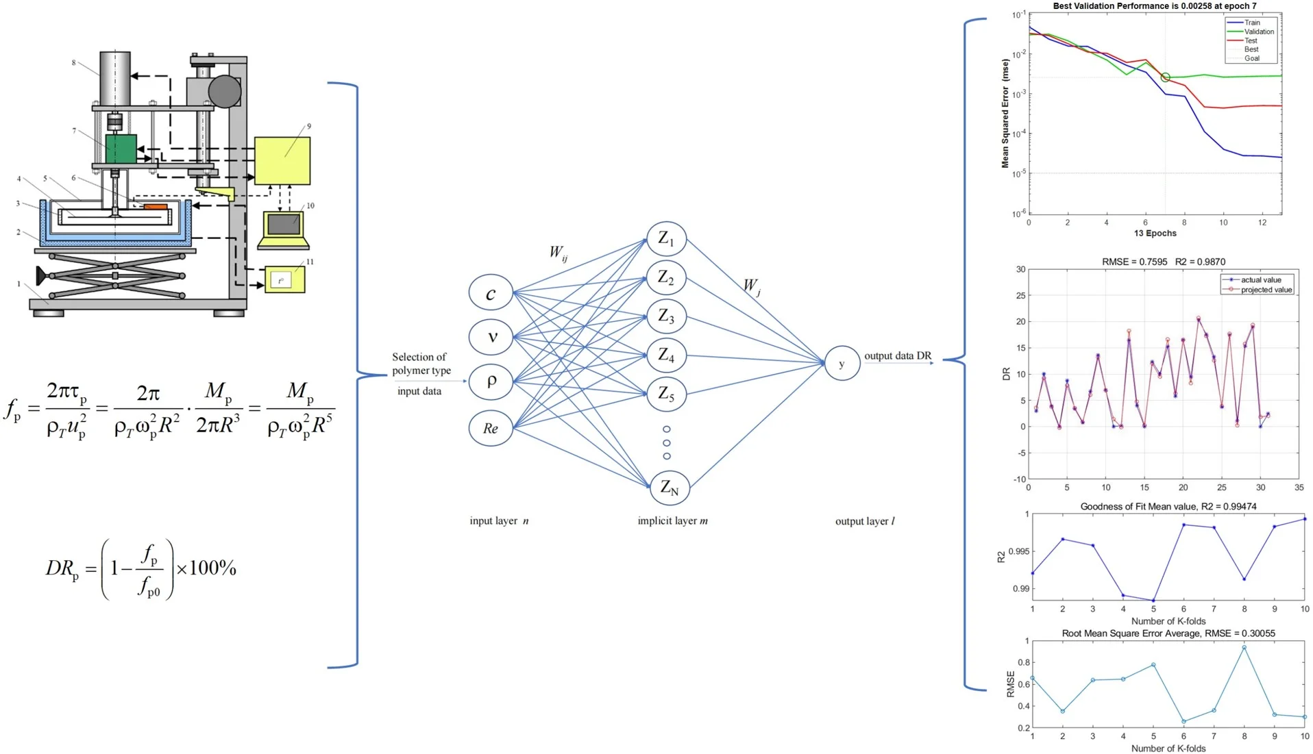
B = \frac{l g (\frac{l g (v_{2} + 0.8)}{l g (v_{1} + 0.8)})}{l g (T_{2} + 273.15) - l g (T_{1} + 273.15)}, A = l g l g (v_{1} + 0.8) - B l g (T_{1} + 273.15) .

Turbulent drag reduction efficiency testing of different polymer drag reducer diesel solutions was carried out based on a flat plate rheological device, the geometry of the device is shown in Fig. 1(a), and the specific physical object is shown in Fig. 1(b). The frictional resistance coefficient $f_{p}$ , and thus the drag reduction efficiency $D R_{p}$ , was obtained by measuring the anti-torque value $M_{p}$ produced by the discs on the polymer oil solution, and then the specific computational expression was calculated as follows:

2

f_{p} = \frac{2 π τ_{p}}{ρ_{T} u_{p}^{2}} = \frac{2 π}{ρ_{T} ω_{p}^{2} R^{2}} \cdot \frac{M_{p}}{2 π R^{3}} = \frac{M_{p}}{ρ_{T} ω_{p}^{2} R^{5}},

3

D R_{p} = (1 - \frac{f_{p}}{f_{p 0}}) \times 100 %,

where $f_{p}$ , $f_{p 0}$ – Fanning’s friction coefficients on the upper and lower surfaces of the discs with and without polymer additive, respectively; $M_{p}$ – anti-torque (N-m); $D R_{p}$ – turbulence reduction efficiency (%) obtained from the tests in the flat plate rheostat.

Fig. 1Flat plate rheostat: 1 – a tripod with a lifting mechanism; 2 – thermostatic bath; 3 – measuring chamber; 4 – rotating disk; 5 – measuring module; 6 – thermometer; 7 – torque sensor; 8 – servomotor; 9 – control and data processing unit; 10 – computer; 11 – thermostat

Flat plate rheostat: 1 – a tripod with a lifting mechanism; 2 – thermostatic bath; 3 – measuring chamber; 4 – rotating disk; 5 – measuring module; 6 – thermometer; 7 – torque sensor; 8 – servomotor; 9 – control and data processing unit; 10 – computer; 11 – thermostat

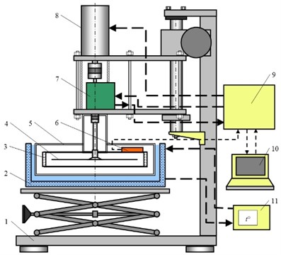
a) Structural diagram

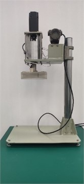
b) Physical drawings

Table 1Properties of polymer resistance reducers by type

Polymer Model	Appearances	Ingredient	Density (kg/m³)	Viscosity (mPa·s)	flash point (℃)	pour point (℃)
FLOXL	Grey suspension	Poly (alpha hexene), poly (alpha octene), poly (alpha dodecane)	860-890 (22 ℃)	≥ 100 (23 ℃)	> 62	–30
FLOМXA	Light white opaque liquid	Poly (alpha hexene), poly (alpha octene), poly (alpha dodecane), alkyl alcohol, 2-methyl-2,4-pentanediol	839 (20 ℃)	800-1000 (20 ℃)	68.89	–30
Necadd-447	Yellow color suspension	Polyalphaoctene	840-900 (20 ℃)	30000-40000 (23 ℃)	> 61	–
М-Flowtreat	Yellowish white suspension	Poly alpha Hexene	840-930 (20 ℃)	1000 (20 ℃); 50000 (40 ℃)	> 63	–50
EP	Pale greyish-white suspension	Polyolefin synthetic rubber, polyacrylamide wax, diethylene glycol butyl ether	850 (20 ℃)	1000 (20 ℃)	> 65	–

The polymer turbulence drag reduction efficiency (DR) under different polymer types, concentrations ( $c$ ), viscosities ( $υ$ ), densities ( $ρ$ ), and Reynolds numbers ( $R e$ ) were obtained based on real-time measurements. Recorded and organized as a data set, the experimental data situation of the four polymer drag-reducing agents is shown in Table 3, and the specific part of the experimental results are shown in Table 2, taking FLOXL as an example.

Table 2Experimental data range and results of four polymer drag-reducing agents

Types of polymers	Concentrations $c$ (ppm)	Viscosities $v$ (mm²/s)	Densities $ρ$ (kg/m³)	Reynolds numbers $R e$	Number of experimental results
FLOXL	0-60	3.67-4.51	825.8-831.5	98199-601961	106
M-Flowtreat	0-60	3.28-4.42	822.3-830.9	112294-675302	113
Necadd-447	0-60	3.23-3.94	821.9-827.8	112294-684223	106
FLO MXA	0-60	3.6-4.42	825.1-831	100114-614575	105

Table 3Results of experimental data for FLOXL drag reducer

Types of polymers	Concentrations $c$ (ppm)	Viscosities $v$ (mm²/s)	Densities $ρ$ (kg/m³)	Reynolds numbers $R e$	DR (%)
FLOXL	0	4.51	831.5	137331	0
FLOXL	0	4.51	831.5	157030	0
FLOXL	5	4.43	831	239789	4
FLOXL	5	4.41	830.9	261086	5.75
FLOXL	10	4.39	830.8	241744	3.4
FLOXL	10	4.37	830.6	263260	5.19
FLOXL	20	4.38	830.7	242706	2.54
FLOXL	20	4.35	830.5	264272	3.95
FLOXL	40	4.4	830.8	241562	2.57
FLOXL	40	4.37	830.7	263208	3.72
FLOXL	60	4.4	830.8	241461	2.61
FLOXL	60	4.39	830.8	262057	4.32

3. BP neural network structure and result prediction

3.1. BP neural network structure

BP Neural Network (Backpropagation Neural Network) is a common artificial neural network model used to solve problems such as pattern recognition and function approximation. It consists of an input layer, a hidden layer and an output layer, each of which consists of multiple neurons (nodes). Each neuron receives input signals and produces output signals, while the connections between them are also given different weights. Through continuous iterative training, BP Neural Networks can learn complex mapping relationships between inputs and outputs and can be used to predict or classify new inputs.

In this paper, a total of four polymer drag reducers are selected, to avoid the data differences caused by the final model accuracy error, while allowing the trained neural network to converge quickly, the data normalization process needs to be carried out on all the data before the training, the data is normalized to the range of the interval of [-1,1], and its computational expression is shown in Eq. (4), and at the same time randomly dividing the dataset into 70 % of the training set and 30 % of the test set:

4

X_{i} = \frac{(a - b) \times (x_{i} - x_{m i n})}{x_{m a x} - x_{m i n}} + b,

where $x_{i}$ is the parameter variables within the data set, i.e., polymer concentration, viscosity, density, Reynolds number, and drag reduction efficiency; $x_{m a x}$ , $x_{m i n}$ are the maximum and minimum values of the data for this experimental sample, respectively; $a$ and $b$ are constants that are taken to be 1 and –1, respectively; and $X_{i}$ is the normalized value of the data set.

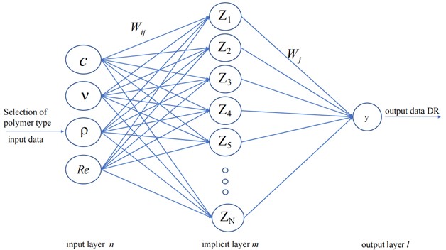
The BP neural network prediction model established in this paper is a three-layer structure, which consists of the input layer, hidden layer, and output layer. The input layer is polymer concentration, viscosity, density, and Reynolds number, and the output layer is polymer drag reduction efficiency. The Tanh function was chosen as the activation function between the input layer and the implied layer, and its computational expression is given in Eq. (5). Between the implied layer and the input layer, the linear function is chosen as the activation function, and its calculation expression is shown in Eq. (6):

5

f (x) = \frac{e^{x} - e^{- x}}{e^{x} + e^{- x}},

6

f (x) = x .

The whole BP neural network selects the trainlm as the training function, and the specific BP neural network structure and parameters are shown in Table 4.

Table 4BP neural network parameters

Project title	Relevant parameters
Number of nodes in the input layer	4
Number of nodes in the output layer	1
Learning rate	0.01
Number of training sessions	1000
Training target accuracy	1.00E-05

In this paper, we set the input parameters of the input layer to be polymer drag reducer concentration ( $c$ ), viscosity ( $υ$ ), density ( $ρ$ ), Reynolds number ( $R e$ ), and the output parameter of the output layer to be polymer turbulence drag reduction efficiency (DR), respectively, and the execution process between the input layer and the implied layer is:

7

m_{j} = φ (\overset{4}{\sum_{i = 1}} ω_{i j} x_{i} + α),

where $j$ is the optimal number of hidden layers; $α$ is the fitting parameter; $φ$ the activation function determined; $ω_{i j}$ is the connection weight between the input layer and the hidden layer.

The specific execution process between the implicit and output layers is:

8

y = φ (\overset{j}{\sum_{k = 1}} ω_{k} m_{k} + β),

where $y$ is the normalized drag reduction efficiency predicted by the neural network; $β$ is the fitting parameter; and $ω_{k}$ is the connection weights between the implicit and output layers.

The specific neural network structure established is shown in Fig. 2.

The $y$ value of the output layer of the BP neural network ranges from [–1, 1], and the output y needs to be reduced to obtain the polymer drag reduction efficiency, as shown in Eq. (9):

9

\overset{∵}{D R_{i}} = \{[(\overset{}{D R} {}_{m a x} - \overset{}{D R} {}_{m i n}) (\overset{}{D R} {}_{i} - b)] / (a - b) + \overset{}{D R} {}_{m i n}\} .

3.2. The number of nodes in the hidden layer is determined

The number of hidden layer nodes will have a large impact on the established polymer turbulence drag reduction efficiency, and because the optimal number of hidden layers corresponding to the data of each polymer is different, to obtain the optimal number of hidden layer nodes of each polymer drag reducer, the range of the number of hidden layer neurons is determined by the number of input and output layers, as shown in Eq. (10):

10

m = \sqrt{n + l} + t,

where, $n$ is the number of neurons in the input layer, $n =$ 4; $m$ is the number of neurons in the hidden layer of the neural network, $m$ takes the range of [4, 13]; $l$ is the number of neurons in the output layer of the neural network, $l =$ 1; and $t$ is a constant in the range of the interval [1, 10].

Fig. 2Structure of BP neural network for prediction of polymer turbulence drag reduction efficiency

To select the optimal number of hidden layer nodes, the root mean square error (RMSE) is chosen as the evaluation index. The BP neural network is trained from the range of the number of neurons in the hidden layer, and the number of hidden layer nodes corresponding to the neural network with the smallest root-mean-square error (RMSE) in the training set is determined as the optimal hidden layer. Where the root mean square error (RMSE) is calculated as shown in Eq. (11):

11

R M S E = \sqrt{\frac{1}{N} \sum_{t = 1}^{N} (p r e d i c t e d_{t} - l a b e l)^{2}} .

Table 5Root mean square error (RMSE) within the number of hidden layers of FLOXL data

Number of neurons in the hidden layer	Normalized root mean square error (RMSE)	Number of neurons in the hidden layer	Normalized root mean square error (RMSE)
4	0.0004231	9	0.0003342
5	0.019318	10	0.0004459
6	0.032353	11	0.0001788
7	0.0015129	12	0.0003119
8	0.0003104	13	0.0005499

Table 6Number of neurons in the optimal hidden layer of polymers

Polymer type	The training set normalized root mean square error (RMSE)	The optimal number of hidden layer neurons
FLOXL	0.000179	11
M-Flowtreat	0.000108	13
Necadd-447	5.63E-05	8
FLO MXA	0.00026	12

The results of the root mean square error (RMSE) within the number of hidden layers corresponding to the FLOXL data are shown in Table 5, from which the optimal number of hidden layer nodes corresponding to the FLOXL polymer is obtained as 11, and the corresponding training set has the smallest normalized root mean square error (RMSE) value of 0.000179. The optimal number of neurons in the hidden layer corresponding to each of the four polymers is obtained by calculating the number of neurons in the hidden layer corresponding to each of the four polymers. The specific results are shown in Table 6.

3.3. Outcome prediction of BP neural networks

Based on the optimal number of hidden layers obtained above, the BP neural network models corresponding to different polymers were established. After the training of the BP neural network is completed, the graphs of the mean square error (MSE) of the four polymer drag reducers with the number of training are obtained, and the optimal validation performance of the four polymer drag reducers during the training process is obtained, and the results are shown in Fig. 3.

Fig. 3Plot of mean square error (MSE) of the polymers with the number of training sessions

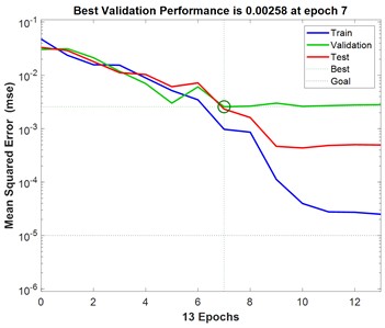
a) FLOXL

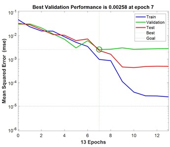
b) FLO MXA

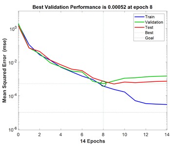
c) Necadd-447

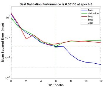
d) M-Flowtreat

Fig. 3 demonstrates the variation of mean square error with increasing number of iterations for predicting BP neural networks for turbulent drag reduction efficiency of different polymer solutions. As can be seen in Fig. 3, the mean square error of the training set, validation set, and test set is larger at the beginning and gradually decreases with the increasing number of iterations of the BP neural network. With the increase in the number of iterations, the change in the mean square error of the three tends to level off, and the location of the small green circle in the figure represents the mean square error at the best number of iterations. To prevent the BP neural network from overfitting and improve the prediction performance of the model, the early stopping strategy that comes with MATLAB is used. The performance of the validation dataset is periodically evaluated during the training process so that the training can be stopped in time when the validation performance stops improving, thus improving the generalization performance of the established BP neural network. In this training process, the early stopping criterion is utilized. When the mean square error of the validation set no longer decreases for six consecutive times and the validation performance does not improve, the training ends, confirming that the BP neural network established at this time is the optimal model. As can be seen in Fig. 3, when the iteration errors of the four polymers FLOXL, М-Flowtreat, Necadd-447, and FLOMXA reached 7, 7, 8, and 6, respectively, the mean-square errors of the validation set converged to the minimum value, which were all less than 10-2, and did not degrade any more in the following six training sessions, which indicated that the BP neural network had reached the convergence condition.

4. Effectiveness evaluation and practical application

4.1. Evaluation of the effect of BP neural network

According to the calculated optimal number of hidden layers, the BP neural network models corresponding to different polymers were established, and the root mean square error (RMSE) value and the goodness of fit $R^{2}$ were chosen as the evaluation indexes to evaluate the prediction effect of the established BP neural network models, and the specific results are shown in Fig. 4.

Fig. 4Comparison of predicted and actual values of BP neural network prediction test set

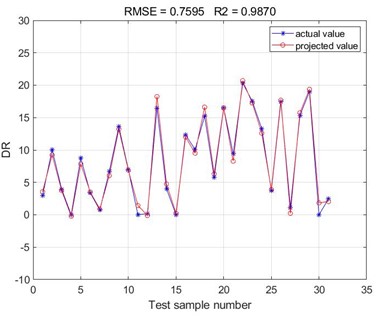
a) FLOXL

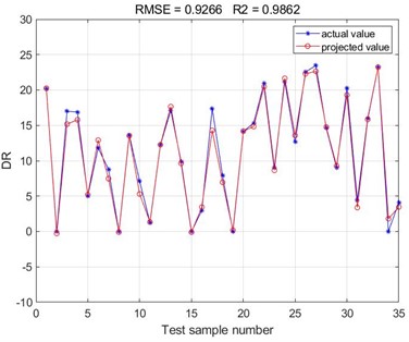
b) FLO MXA

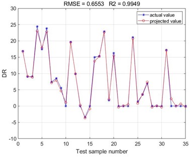
c) Necadd-447

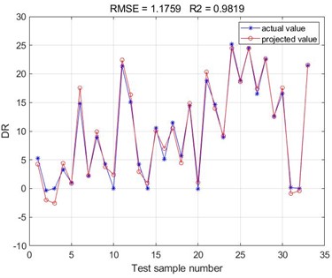
d) M-Flowtreat

According to the results of the comparison between the test set of BP neural network predictions obtained from the training of the four polymer drag reduction and the actual values, it can be seen that the results predicted by the BP neural network are consistent with the results of the polymer turbulence drag reduction efficiency measured by the experiment. The root mean square error (RMSE) values of the BP neural networks obtained from this training are all below 2, and the goodness of fit $R^{2}$ is above 0.98. Since the Root Mean Square Error (RMSE) values reflect the deviation between the predicted and true values and are more sensitive to outliers in the data. Accordingly, it can be concluded that the accuracy of the present method in predicting the polymer turbulence drag reduction efficiency is high, indicating a good fitting of the correlation of the selected sample data set. The drag reduction performance of the four polymer drag reduction types can be predicted using the trained BP neural network model. It can be seen that there is a good correlation between the basic parameters such as polymer drag-reducing agent type, concentration, viscosity, density, Reynolds number, and polymer drag-reduction efficiency. Meanwhile, the root mean square error (RMSE) values and the goodness of fit $R^{2}$ values obtained from the four polymer drag reduction BP neural networks are compared. It can be found that the BP neural network obtained from the training of the Necadd-447 model of drag-reducing agent has the best prediction with the smallest Root Mean Square Error (RMSE) value of 0.6553 and the largest $R^{2}$ value of goodness of fit of 0.9949.

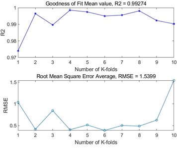
Fig. 510-fold cross-validation results of four polymer BP neural networks

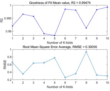
a) FLOXL

b) FLO MXA

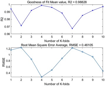
c) Necadd-447

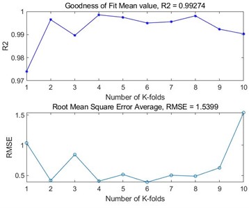
d) M-Flowtreat

In order to further assess the generalisation ability of the BP neural network models and to detect the overfitting of the models, the evaluation of the BP neural network models built by the four polymers was further carried out using $K$ -fold cross-validation. By dividing the dataset into $K$ similarly sized subsets, using $K - 1$ of them as the training set each time, and the remaining one as the validation set, and repeating the process $K$ times, $K$ independent model performance evaluations were obtained, and finally, the performance metrics of the $K$ times were averaged as the final evaluation results of the model. In this $K$ -fold cross-validation, we take the value of $K$ as 10, and choose the root mean square error and goodness of fit as the evaluation metrics to evaluate the four polymer models, and the results are shown in Fig. 5. From the figure, it can be seen that the BP neural networks established by the four polymers have good prediction accuracy in the case of 10-fold cross-validation, the average value of the goodness of fit is above 0.98, and the average value of the root mean square error is below 2. Based on the results of the 10-fold cross validation, it can be seen that the established BP neural network model is accurate and stable, and at the same time, it performs well on the whole dataset, and there is no overfitting.

4.2. Long-distance pipeline applications for refined oil products

Based on the above evaluation of the polymer turbulence drag reduction efficiency prediction results, it can be seen that the BP neural network has a high prediction accuracy for the experimental results, and can play an obvious prediction advantage in the field of polymer turbulence drag reduction. To further verify and improve the accuracy of the prediction model, based on the established BP neural network prediction model, it is applied in the turbulence-damping transport process of industrial oil products pipeline and then realizes the prediction of turbulence-damping efficiency of long-distance oil products transport pipeline. In this paper, we use M-FLOWTREAT polymer drag reducer with the concentration of $c =$ 4.91-15.06 ppm, diesel viscosity of $υ =$ 7.5 mm²/s, and density of $ρ =$ 843.6-847.8 kg/m³ to carry out turbulence reduction experiments on the long-distance oil product pipeline of the section Vtorovo-Primorsk, with the length of the pipeline $L =$ 227 km and the diameter of the pipeline $D =$ 530 mm. Turbulence drag reduction experiments are carried out in the oil pipeline, and a BP neural network prediction model is established based on the obtained drag reduction flow data.

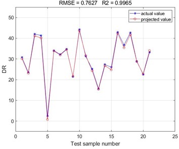
The pipeline operation dataset is imported into MATLAB software, which is also randomly divided into 70 % of the training set and 30 % of the test set. The BP neural network was established, and the prediction accuracy and root mean square error of the BP neural network were compared and analyzed under the conditions of different numbers of hidden layer neurons. The optimal number of hidden layer neurons is selected as 13, and the optimal BP neural network model is established. Based on the established model, the polymer turbulence drag reduction efficiency is predicted, and the specific prediction fitting results are shown in Fig. 6. Comparative analysis of the predicted and actual values of the BP neural network prediction test set for M-FLOWTREAT refined oil pipeline shows that the BP neural network established based on the data set of polymer drag reducer type, concentration ( $c$ ), viscosity ( $υ$ ), density ( $ρ$ ), and Reynolds number ( $R e$ ) can accurately predict turbulence damping efficiency of the pipeline with the addition of the polymer drag reducer, and the goodness of fit of the BP neural network model is up to 0.9965.

Fig. 6Comparison of predicted and actual values of M-FLOWTREAT refined oil pipeline prediction test set

Since the long-distance pipeline transport of refined oil products is a closed sequence transport, with the change of polymer damping agent type, injection volume, and pipeline operation state, the turbulence damping efficiency of the polymer damping agent will produce corresponding changes. Using the BP neural network, the turbulence-damping efficiency of the polymer damping agent can be predicted quickly, so that the pumping station in the pipeline conveying process can be reasonably regulated. However, the influencing factors of polymer turbulence damping efficiency are complex and related to polymer concentration, viscosity, density, molecular weight, pipeline flow parameters, etc. The BP neural network prediction model cannot completely replace the experimental test, but rather, through the database accumulated in the past, it can quickly react to the unknown state and obtain the new polymer damping efficiency, which can help the daily management of the pipeline transportation of refined oil products and reduce the energy consumption.

5. Conclusions

Since polymer-reducing agents can greatly reduce the operating cost of long-distance pipeline transport of refined oil products, this paper proposes and establishes a polymer turbulence drag-reducing efficiency prediction model based on the BP neural network according to the basic parameters of polymer drag-reducing agents and different working conditions of pipeline operation.

1) Based on the data from the polymer turbulence drag reduction experimental system, the polymer type, polymer concentration, viscosity, density, and Reynolds number are selected as the influencing factors. The root mean square error is used as the evaluation index to determine the optimal number of neurons in the hidden layer for different polymers and the optimal BP neural network prediction model for different polymer drag reducers is obtained.

2) The established BP neural network model was used to predict the polymer drag reduction efficiency, and the root mean square error (RMSE) values of the predicted and actual values were compared and analyzed, as well as the goodness-of-fit $R^{2}$ . The results of the effect evaluation showed that the predicted values of the BP neural network and the actual distribution of the data on the drag reduction efficiency were the same, and the BP neural network fitting accuracies for the four types of polymer drag reducers were all above 0.98. Among them, the Necadd-447 model was the best fitted, with a goodness-of-fit $R^{2}$ of 0.9949. The model was also evaluated using 10-fold cross-validation, and based on the results, it can be seen that the established BP neural network model is accurate and stable, and at the same time performs well on the entire dataset without overfitting.

3) BP neural network is applied to predict the long-distance oil pipeline of refined oil products with the addition of polymer. The results show that the goodness of fit $R^{2}$ can reach 0.9965, and the turbulence damping efficiency of polymer damping agent can be predicted quickly, to reasonably regulate the pumping station in the process of pipeline transmission and reduce the energy consumption in the process of refined oil pipeline transmission.

References

B. A. Toms, “Some Observations on the flow of linear polymer solutions through straight tubes at large Reynolds numbers,” in First International Congress on Rheology, 1948.

Search CrossRef
D. Mowla and A. Naderi, “Experimental study of drag reduction by a polymeric additive in slug two-phase flow of crude oil and air in horizontal pipes,” Chemical Engineering Science, Vol. 61, No. 5, pp. 1549–1554, Mar. 2006, https://doi.org/10.1016/j.ces.2005.09.006

Publisher
S. N. Shah, Ahmed Kamel, and Y. Zhou, “Drag reduction characteristics in straight and coiled tubing – An experimental study,” Journal of Petroleum Science and Engineering, Vol. 53, No. 3-4, pp. 179–188, Sep. 2006, https://doi.org/10.1016/j.petrol.2006.05.004

Publisher
Q. Quan et al., “Experimental study on the effect of high-molecular polymer as drag reducer on drag reduction rate of pipe flow,” Journal of Petroleum Science and Engineering, Vol. 178, pp. 852–856, Jul. 2019, https://doi.org/10.1016/j.petrol.2019.04.013

Publisher
H. J. Choi, C. A. Kim, and M. S. Jhon, “Universal drag reduction characteristics of polyisobutylene in a rotating disk apparatus,” Polymer, Vol. 40, No. 16, pp. 4527–4530, Jul. 1999, https://doi.org/10.1016/s0032-3861(98)00869-6

Publisher
K. Hornik, M. Stinchcombe, and H. White, “Multilayer feedforward networks are universal approximators,” Neural Networks, Vol. 2, No. 5, pp. 359–366, Jan. 1989, https://doi.org/10.1016/0893-6080(89)90020-8

Publisher
H. Wang, Z. Lei, X. Zhang, B. Zhou, and J. Peng, “A review of deep learning for renewable energy forecasting,” Energy Conversion and Management, Vol. 198, p. 111799, Oct. 2019, https://doi.org/10.1016/j.enconman.2019.111799

Publisher
G. B. Goh, N. O. Hodas, and A. Vishnu, “Deep learning for computational chemistry,” Journal of Computational Chemistry, Vol. 38, No. 16, pp. 1291–1307, Jun. 2017, https://doi.org/10.1002/jcc.24764

Publisher
H. Salehi and R. Burgueño, “Emerging artificial intelligence methods in structural engineering,” Engineering Structures, Vol. 171, pp. 170–189, Sep. 2018, https://doi.org/10.1016/j.engstruct.2018.05.084

Publisher
Rene Y. Choi, Aaron S. Coyner, Jayashree Kalpathy-Cramer, Michael F. Chiang, and J. Peter Campbell, “Introduction to machine learning, neural networks, and deep learning,” Translational Vision Science & Technology, Vol. 9, No. 2, Feb. 2020, https://doi.org/10.1167/tvst.9.2.14

Publisher
C. Lee, J. Kim, D. Babcock, and R. Goodman, “Application of neural networks to turbulence control for drag reduction,” Physics of Fluids, Vol. 9, No. 6, pp. 1740–1747, Jun. 1997, https://doi.org/10.1063/1.869290

Publisher
L. V. Lorang, B. Podvin, and P. Le Quéré, “Application of compact neural network for drag reduction in a turbulent channel flow at low Reynolds numbers,” Physics of Fluids, Vol. 20, No. 4, Apr. 2008, https://doi.org/10.1063/1.2904993

Publisher
J. Park and H. Choi, “Machine-learning-based feedback control for drag reduction in a turbulent channel flow,” Journal of Fluid Mechanics, Vol. 904, p. A24, Dec. 2020, https://doi.org/10.1017/jfm.2020.690

Publisher
B.-Z. Han and W.-X. Huang, “Active control for drag reduction of turbulent channel flow based on convolutional neural networks,” Physics of Fluids, Vol. 32, No. 9, Sep. 2020, https://doi.org/10.1063/5.0020698

Publisher
K. Fukami, Y. Nabae, K. Kawai, and K. Fukagata, “Synthetic turbulent inflow generator using machine learning,” Physical Review Fluids, Vol. 4, No. 6, p. 064603, Jun. 2019, https://doi.org/10.1103/physrevfluids.4.064603

Publisher
H. Moayedi, L. K. Foong, and H. Nguyen, “Soft computing method for predicting pressure drop reduction in crude oil pipelines based on machine learning methods,” Journal of the Brazilian Society of Mechanical Sciences and Engineering, Vol. 42, No. 11, pp. 1–11, Nov. 2020, https://doi.org/10.1007/s40430-020-02613-x

Publisher
H. Moayedi, B. Aghel, B. Vaferi, L. K. Foong, and D. T. Bui, “The feasibility of Levenberg-Marquardt algorithm combined with imperialist competitive computational method predicting drag reduction in crude oil pipelines,” Journal of Petroleum Science and Engineering, Vol. 185, p. 106634, Feb. 2020, https://doi.org/10.1016/j.petrol.2019.106634

Publisher

About this article

Received

26 September 2023

Accepted

12 October 2023

Published

30 October 2023

DOI

https://doi.org/10.21595/lger.2023.23661

Keywords

turbulent drag reduction

polymer

BP neural network

efficiency prediction

pipeline transportation

Acknowledgements

We would like to acknowledge support from assistance from Ufa State Petroleum Technological University and Southwest Petroleum University. This work was supported by the National Natural Science Foundation of China (No. 52004241), the Natural Science Foundation of Sichuan Province (No. 2022NSFSC1018), the Open Fund Project of SINOPEC Key Laboratory for EOR of Fractured-vuggy Reservoir (34400000-22-ZC0607-0006).

Data Availability

The datasets generated during and/or analyzed during the current study are available from the corresponding author on reasonable request.

Author Contributions

Yang Chen: conceptualization, formal analysis, funding acquisition, investigation, resources, software, supervision, validation, writing – review and editing. Minglan He: data curation, investigation, methodology, project administration, software, visualization, writing – original draft preparation. Meiyu Zhang: formal analysis, methodology, project administration. Jin Luo: project administration.

Conflict of interest

The authors declare that they have no conflict of interest.

This is an open access article distributed under the Creative Commons Attribution License, which permits unrestricted use, distribution, and reproduction in any medium, provided the original work is properly cited.

Previous article in issue Previous

Research article

2023 10 20

Structural seismic response prediction based on convolutional neural networks

Feiyu Guo, Yinfeng Dong, Hui Tian, Xingyu Zhang, Qingshuang Su

Research article

2021 12 02

Research on prediction method of section convergence and deformation of shield tunnel in operation period based on deep learning

Fei Sun, Haolong Zheng, Changjun Li

Research article

2019 11 15

Chaotic time series prediction using wavelet transform and multi-model hybrid method

Tian Feng, Shuying Yang, Feng Han

Research article

2019 06 30

Research on aero-engine fault diagnosis based on integrated neural network

Shi Xiangyang

Y. Chen, M. He, M. Zhang, and J. Luo, “Prediction and evaluation of polymer turbulent drag reduction efficiency based on BP neural network,” Liquid and Gaseous Energy Resources, Vol. 3, No. 2, pp. 76–88, Oct. 2023, https://doi.org/10.21595/lger.2023.23661

Copy Extrica

Copied to clipboard!

TY  - JOUR
DO  - 10.21595/lger.2023.23661
UR  - https://doi.org/10.21595/lger.2023.23661
TI  - Prediction and evaluation of polymer turbulent drag reduction efficiency based on BP neural network
T2  - Liquid and Gaseous Energy Resources
AU  - Chen, Yang
AU  - He, Minglan
AU  - Zhang, Meiyu
AU  - Luo, Jin
PY  - 2023
DA  - 2023/10/30
PB  - JVE International Ltd.
SP  - 76-88
VL  - 3
IS  - 2
SN  - 2669-2791
ER  - 

Copy Ris

Copied to clipboard!

 @article{Chen_2023, title={Prediction and evaluation of polymer turbulent drag reduction efficiency based on BP neural network}, volume={3}, ISSN={2669-2791}, url={https://doi.org/10.21595/lger.2023.23661}, DOI={10.21595/lger.2023.23661}, number={2}, journal={Liquid and Gaseous Energy Resources}, publisher={JVE International Ltd.}, author={Chen, Yang and He, Minglan and Zhang, Meiyu and Luo, Jin}, year={2023}, month=oct, pages={76–88} }

Copy Bibtex

Copied to clipboard!

[1]Y. Chen, M. He, M. Zhang, and J. Luo, “Prediction and evaluation of polymer turbulent drag reduction efficiency based on BP neural network,” Liquid and Gaseous Energy Resources, vol. 3, no. 2, pp. 76–88, Oct. 2023, doi: 10.21595/lger.2023.23661.

Copy IEEE

Copied to clipboard!

Chen, Yang, Minglan He, Meiyu Zhang, and Jin Luo. “Prediction and Evaluation of Polymer Turbulent Drag Reduction Efficiency Based on BP Neural Network.” Liquid and Gaseous Energy Resources 3, no. 2 (October 30, 2023): 76–88. https://doi.org/10.21595/lger.2023.23661.

Copy Chicago

Copied to clipboard!

Prediction and evaluation of polymer turbulent drag reduction efficiency based on BP neural network

Abstract

Highlights

1. Introduction

2. Experiments and methods

3. BP neural network structure and result prediction

3.1. BP neural network structure

3.2. The number of nodes in the hidden layer is determined

3.3. Outcome prediction of BP neural networks

4. Effectiveness evaluation and practical application

4.1. Evaluation of the effect of BP neural network

4.2. Long-distance pipeline applications for refined oil products

5. Conclusions

References

About this article

Related Articles