Estimating the frequencies of vibration signals using a machine learning algorithm with explained predictions

1. Introduction

Analyzing the signals in the frequency domain is a common practice in structural health monitoring (SHM), which has proved its reliability [1]. Although the procedure seems simple, the accuracy of the results is unsatisfactory by applying standard methods such as DFT or FFT [2]. The low accuracy is achieved because the vibration signals resulting from impulsive excitation are short and contain few vibration cycles. Numerous researchers have tried to introduce interpolation methods to improve the estimation results and consequently obtain frequencies with a high level of precision [3]-[7]. A systematic review of these methods, which also quantify errors concerning the signal length, is presented in [8]. Zero-padding is a viable alternative to interpolation [9]. Trim-to-fit methods are also used for more accurate frequency estimation [2], [11]. However, the methods mentioned above do not yield highly accurate results.

This paper presents a method to estimate the frequencies based on the discrete Fourier Transform (DFT) property to produce systematically repeatable errors and a method involving artificial neural networks (ANN). In addition to other existing frequency estimation methods, this network also provides information regarding the accuracy of the estimation.

2. The origin of errors in standard frequency estimation

An analog sinusoidal signal has its time history $a\left(t\right)$ expressed as follows:

In Eq. (1), $A$ is the signal amplitude, $f_R$ is the signal frequency, and $t$ is the length of the signal in the time domain. In the digital form, when sampling the signal with a sampling rate $f_S$ and using $N$ samples, the signal becomes a sequence:

Applying a standard DFT, the sequence $a\left[n\right]$ is converted in the frequency domain. It results in $N$ amplitudes displayed on spectral lines $k$ numbered from 0 to $N$–1. The value calculated for the $k$-th line is:

Every $A_k$ can be decomposed into a real part $\mathit{Re}{A}_k$, and an imaginary part $\mathit{Im}{A}_k$, as follows:

In consequence, the $k$-th spectral line will display the magnitude:

The spectral lines on which the amplitudes are displayed are equidistant. The distance between them is nominated as the frequency resolution. It is calculated according to the expression:

If $f_R$ is a multiple of the frequency resolution $∆f$, thus:

with $k$ as a natural number, the true frequency is located on one of the spectral lines. At that spectral line, the actual amplitude $\left|M_k\right|$ of the signal will be displayed. The displayed amplitudes are zero on all other lines, meaning the true frequency was found. In Figure 1, we represent with red color the spectral line on which the true frequency is located.

The abovementioned case corresponds to the case where the signal has an integer number of cycles. It means the time length $t$ is a multiple periods $T$ of the sinusoidal signal. We can deduce this from the reversed Eqs. (7) and (8). These are:

Now, from Eq. (9), it directly results that:

Fig. 1The DFT represents a sinusoidal signal. The spectral lines for the standard DFT are represented with red lines having squares with a red contour on the tip; the additional squares represent the amplitudes of the supplementary spectral lines obtained by zero-padding (dashed lines); the magenta line with a blue square on the tip is associated with the actual frequency and is located on an inter-line position

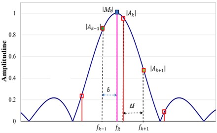
Hence, the spectral line number indicates the number of cycles present in the signal for the harmonic component with frequency $f_R$. If k is not an integer, $f_R$ will be located at an inter-line position due to the positions of the spectral lines defined by the time length $t$. In this case, the displayed amplitude is $A_k$, smaller than the actual amplitude of the signal. Moreover, amplitudes will also be displayed on other spectral lines. On the neighbor spectral lines of $k$, these amplitudes are $A_{k-1}$ and $A_{k+1}$, plotted with a square having a red contour in Figure 1.

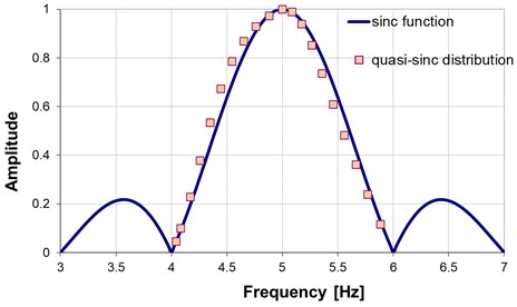
The distribution of $A_k$ when modifying the time length of the sinusoidal signal is quasi a $\mathrm{s}\mathrm{i}\mathrm{n}\mathrm{c}$ function (Figure 2) centered on the real frequency or its spectral line if the spectrum is constructed using this approach. In order to have more points in the spectrum, we can lengthen the signal by adding points with zero amplitude, the so-called zero-padding [9]. If we double the number of samples, we obtain twice more spectral lines. The new amplitudes in the DFT represented in Figure 1 are marked with green squares with a red contour.

Fig. 2Comparison between the (quasi-sinc) distribution of Ak and the sinc function

One can observe in Figure 1 that the more dense spectral lines provide a better image of the shape of the $\mathrm{s}\mathrm{i}\mathrm{n}\mathrm{c}$ function. We can also observe that the distance between the frequency displayed at line $k-1$ (i.e., $f_{k-1}$) and $f_R$ is the so-called correction term $\delta$. We can write:

Hence, the normalized correction term can be calculated with the mathematical relation:

The following section proposes finding the correction term using an ANN model.

3. The methodology to create the ANN model and estimate correctly the frequency

The ANN is destined to find the correction term $\delta$. The first step in developing the ANN model is to generate a sinusoidal signal with known frequency and amplitude. Using this signal, we develop a database containing the frequencies $f_{k-1}$, $f_{k1}$, $f_{k+1}$ and the associated amplitudes $A_{k-1}$, $A_{k1}$, $A_{k+1}$, obtained using the DFT algorithm for different signal lengths. The crop is made by extracting two samples at iteration. For each set of data, we also calculate the correction term $\delta$.

The generated sinusoidal signal has the amplitude $A$ = 1 and the frequency $f_R$ = 5 Hz. It is zero-padded to double its length. Initially, the entire signal has $N_{max}$ = 2155 samples taken by a frequency rate of $f_S$ =1000 Hz. Two samples are extracted by iteration, one from the sinusoid and one from the zero-padded end until the signal contains $N_{min}$ = 1925 samples. The longest signal time length is $t_{max}$ = 2.154 s, and the shortest is $t_{min}$ = 1.924 s. Figure 3 represents the amplitudes $A_k$ obtained in the DFT spectrum. We can observe the pattern for each cycle of time length $T$. The amplitudes decrease with each cycle because less energy is contained in the shorter signal.

Fig. 3The amplitude Ak obtained for the signal by applying a standard DFT; the limits of the portion extracted for training are marked with arrows

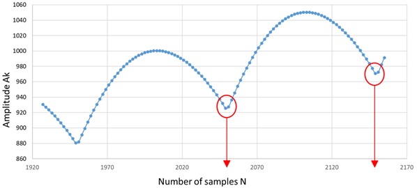
Based on the repeatability, it is enough to consider the data obtained by cropping one cycle, thus having a time length between $k$ – 0.5 (a minimum in the diagram in Figure 3) and $k$ + 0.5 (the following minimum in the diagram in Figure 3). So, we extract the portion of data contained between 2149 and 2051 samples. Aiming for the generalization, we do the following:

1. We normalize the amplitudes $A_{k-1}$, $A_{k1}$, and $A_{k+1}$ obtained at each iteration by dividing them with the biggest amplitude $A_{k1}$ achieved in the selected data set;

2. We normalize the calculated correction coefficient $\delta$ with the frequency resolution $\Delta f$ for each iteration separately.

An example of data with highlights on the training data (three input neurons and one output neuron) is given in Table 1.

With the data generated using the above procedure, we train a feed-forward backpropagation neural network with the architecture and main meta-parameters described in Figure 4.

Fig. 4Description of the deep neural network

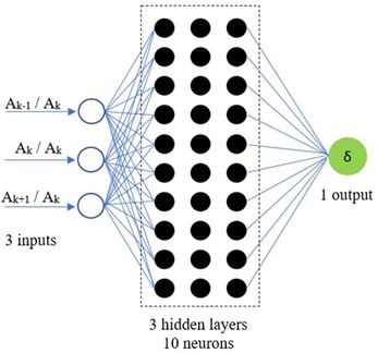
a) The network architecture

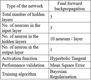
b) The main meta-parameters of the network

To avoid the phenomenon of network overfitting, we train the network by using the Bayesian Regularization function. The performance of the ANN reflected in the regression coefficients obtained after training is as follows: for Training and Validation 0.99847; for Test 0.997316; for the Cumulative data 0.9981. It means we obtained an excellent trained network.

After estimating the normalized correction term $\stackrel{-}{\delta }$ with the ANN model, we calculate the (estimated) frequency $f_O$ using the mathematical relation:

However, to explain why the prediction was made and if it is trustworthy, we add a follow-up to the standard use of the network. This step consists of the following:

1. Calculus of the period $T_O$ that corresponds to $f_O$;

2. Calculus of the signal length $t_O$ by multiplying $T_O$ with k;

3. Calculus of $2k$ the amplitudes in the DFT of the reconstructed sinusoidal signal with length $t_O$ and frequency $f_O$;

4. Calculus of the signal-to-noise ratio.

The signal-to-noise ratio is used to prove the trustworthiness of the prediction. We calculate this parameter with the mathematical relation:

In Eq. (13), $M_k$ is the largest amplitude in the DFT with the length $k{T}_O$. The sum representing the denominator in Eq. (13) is the energy spread on the first $2k$ spectral lines. The bigger the ratio, the better the frequency estimation. In the ideal case, $SNR$ = 1.

4. Validation of the proposed methodology

For validation, we use the original signal described at the beginning of Section 3. We calculate the amplitudes displayed at the first 24 spectral lines and identify the maximizer $M_k$. The spectrum is presented in Figure 5 with a red line, and the relevant data regarding the signal and its DFT is given in Table 2.

Fig. 5The DFT of the original signal (red line) and truncated signal (blue line)

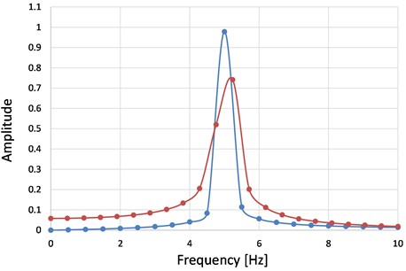
Afterward, we double the length of the signal by zero-padding and estimate the correction term δ involving the trained ANN. With this correction term, we calculate with Eq. (13) the fine estimation of the frequency, which is $f_O$. It follows the calculus of $T_O$ and that of the length of the new signal with an entire number of cycles. The spectrum of this signal is represented in Figure 5 with a blue line. It is easily observable that the amplitudes in the red spectrum are spread along all spectral lines. Dissimilar, the blue spectrum is concentrated around the spectral line displaying the correct frequency, and on all other spectral lines, the amplitudes are small.

Table 2 presents the relevant data regarding the shortened signal and its DFT. We can observe that the fine estimation of the frequency is highly accurate, and the $SNR$ is significantly bigger for the signal with the tuned length calculated following $f_O$. Therefore, the SNR is a clear indicator of the estimation accuracy, and it can be used to explain the decision of the AI system.

5. Conclusions

Automatic decision systems that rely on Artificial Intelligence must prove their decisions to be accepted by humans without hesitation. Thus, in addition to the results, the AI system should accompany the decision with data that a human can interpret. In this study, we show how the frequency estimation of signals can be improved by involving a machine-learning algorithm and propose using the SNR in a follow-up procedure to justify the decision.

Following the numerous experiments performed, one of which we presented in the paper, we noticed that the SNR is always the highest in the case of the correct frequency estimation. For even greater credibility, the system can be adjusted to calculate two more SNRs for a signal slightly more extended and one slightly shorter than the one considered correct. Both SNRs must present lower values than the SRN calculated for the correct estimation.

On the other hand, we demonstrated that using a Machine Learning algorithm, the frequency of the harmonic components of a signal can be estimated with excellent accuracy.

Future concerns will focus on estimating the frequencies of a signal with two close harmonic components.