Abstract
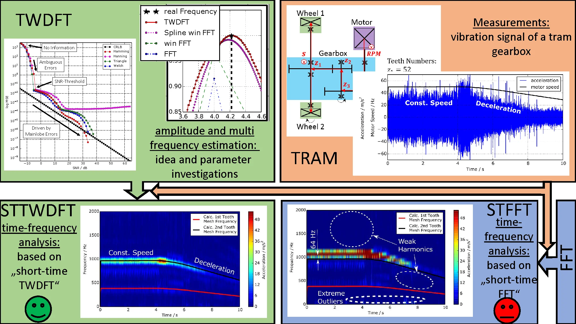
Sinusoidal parameter estimation for determining frequency position and amplitude is challenging for noisy short vibration signals, e.g. from machines or human vibrations. In this paper, we propose the “Trimmed Window Discrete Fourier Transform” (TWDFT) estimator, which uses for every frequency a one-point discrete Fourier transform (DFT) to determine the corresponding spectral amplitude. To avoid leakage effects, it cuts the time interval so that it corresponds to an integer number of period durations. To evaluate the estimator performance, we compare it with relevant estimators such as the Cramer-Rao lower bound (CRLB) and the spectral spline interpolation applied on a noisy mono-frequent test signal with a fractional frequency. For the estimated parameters, the mean squared errors (MSE) are calculated and compared as a function of the signal-to-noise ratio (SNR). The advantages of the TWDFT estimator can be seen over the whole SNR range. The TWDFT estimates are better than the fast Fourier transform (FFT) starting at a SNR of –6 dB. At a SNR of 30 dB, the estimator meets the real value of the frequency and reaches similar results as the CRLB. The application of the TWDFT estimator as a short-time analysis on a vibration signal of a tram gearbox shows a significantly more differentiated time-frequency analysis compared to a short-time Fourier transform (STFT).
Highlights
- New approach for amplitude and multi frequency estimation.
- High accuracy time-frequency analysis of the vibration signal of a tram gearbox.
- Cramer-Rao lower bound.
1. Introduction
The estimation of the correct frequencies and amplitudes of spectral information is necessary for realizing a frequency analysis and estimate the signal power (amplitude) of multi-frequency signals. Such estimators are essential in vibration-based machine diagnostics [1, 2]. Kinematic damage frequencies, e.g. from rolling bearings and gears, are investigated to detect a specific damage. Thereby a more differentiated diagnosis can be realized based on the exact frequency position with respect to time. Last but not least more effective countermeasures for damage prevention can be done.
In literature, a large number of estimation methods for the frequency position and amplitude are available after performing a DFT or FFT, for example the interpolation or iterative interpolation between 3 to 5 discrete neighbouring spectral lines [3-13]. Further scientific works solve the estimation problem by means of iterative optimization methods [14-20] and still others use model based methods, e.g. by estimating the order of the model [13, 21, 22]. In case of multi-frequent and noisy signals, a DFT-based iterative approximation algorithm can be applied for the detection of spectral components [23]. Thereby a model order estimation should be carried out to determine the relevant number of frequencies with a certain risk that undetected frequencies can be interpreted as noise components [13]. Other approaches such as the Chirp-Z transform (CZT) or the ZoomFFT (ZFFT) are narrow-band analysis techniques [24-26], which are computational efficient and estimate therefore the spectrum during the spectral calculation process. The ZFFT realizes the same frequency resolution as the standard FFT, even if it is calculated based on a shorter time signal segment. The short signal segment is generated from the original signal by a simple decimation, which reduces the maximal bandwidth around a selectable centre frequency. Both CZT and ZFFT achieve an improvement in frequency estimation, but are limited in terms of frequency resolution and they can only calculate a small portion of the entire spectrum around the centre frequency [27, 28].
Another approach for spectrum estimation uses integer periodic segments of mono-frequent signals. The segment length is optimized by an iterative search for one instantaneous specific signal frequency [29] followed by an FFT. These methods are used to analyse harmonic power signals [30-32].
However, the problem generally lies in the time-frequency resolution when performing a time-frequency analysis, such as the short-time Fourier transform (STFT). A low frequency resolution is realized due to the short signal segments, so that a sinusoidal parameter estimation is required to improve the time-frequency correspondence [1]. Large signals are thereby split into many small segments, which are subjected to a discrete Fourier transform (DFT) or fast Fourier transform (FFT) to calculate the amplitude spectrum. Typically, these short segments reduce the resolution in the frequency domain, so that a deviation occurs in the calculation of the frequency position and the corresponding amplitude with respect to the true sinusoidal parameters [33]. In the frequency domain, if there is an interesting frequency within the resolution interval, it becomes impossible to calculate it. Furthermore, in most cases the occurring and random frequencies are not a multiple of the frequency resolution in the amplitude spectrum, which is not practical. In Eq. (1), the distance between two spectral lines is described as the reciprocal value of the signal duration :
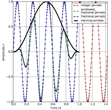
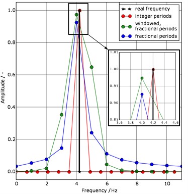
Fig. 1a) Mono-frequent signals (f= 4.2 Hz, fS = 280 Hz) with integer periods (red, N= 400), fractional number of periods (blue, N= 280), fractional number of periods with Hanning window (green, N= 280) and the Hanning window itself (black); b) corresponding amplitude spectra of the three signals (red, blue, green) and the real signal frequency (black)
a)
b)
Another source of inaccuracy are the aperiodic properties of finite and multi-frequency signals. This non-integer “abort” of the signal periods leads to a smearing of the amplitude spectrum in the so called leakage effect [33]. Thereby the amplitude calculation is not correct since the missing components are spread to neighbouring spectral components. Nevertheless, the use of various window functions reduces the leakage effect. For this purpose, an exemplary data set for the visualisation of the mentioned signal theoretical basics is presented in Fig. 1. The blue signal is non-windowed and it has a fractional number of periods. After applying the FFT algorithm the frequency = 4.2 Hz is not computed correctly with regard to its position and amplitude. The reasons for this are the limitations due to the signal time and the leakage effect. In comparison, the same signal is evaluated using the Hanning window (green), which is suitable for a large number of cases. The calculation of the left and right amplitudes for the same signal frequency is more accurate. Nevertheless, a reduction of the leakage effect around the frequency of 4 Hz is observed. This is recognizable by the lower side lobes (from 2 Hz to 6 Hz), which is associated with the broadening of the main lobe.
If the mono-frequency signal has an integer period (Fig. 1(a), red signal), the calculation of the amplitude and the frequency in Fig. 1(b) is exact since the reciprocal value of the signal duration ( 1.43 s, at a sampling frequency = 280 Hz and a sample number = 400) is an integer divider of the searched signal frequency. The leakage effect does not occur because the frequency corresponds to a multiple of the discrete frequency resolution . For multi-frequency signals only one fundamental frequency and its harmonics form the multiple of the discrete frequency step.
The main contribution of this article is the introduction of a new estimator for sinusoidal parameters and its test on real noisy multi-frequency vibration signals of a tram gearbox for accurate time-frequency analyses. For this we propose to overcome these resolution problems by increasing the resolution in the frequency domain together with a frequency-dependent integer periodic signal trimming. The article is divided into three main parts. In chapter 2, the approach for estimating the frequency and amplitude of aperiodic and multi-frequency signals is presented. By using a uniform data set, a simulation study is presented in chapter 3 to investigate the influence of the window functions on the estimated results concerning frequency and amplitude. For this purpose, the mean squared error (MSE) of the developed estimator is compared with conventional estimators. These are, e.g. the Cramer-Rao lower bound (CRLB) [3-6], [27, 28] and [34, 35], which represents the lower limit for the MSE of an estimator and the spline interpolation of at least two spectral lines. In chapter 4, the estimator is applied to real vibration signals of a tram gearbox to evaluate its performance in practice. For this purpose we compare 2 time-frequency analyses, where one is based on STFT and the other is based on short-time TWDFT. To validate the estimation results, the time-dependent courses of the tooth mesh frequencies in the spectrograms are compared with the courses of the tooth mesh frequencies calculated from speed measurement data and gear teeth number. Finally, we provide a summary and an outlook.
2. TWDFT: trimmed window discrete Fourier transform
In this section, we introduce a novel method for sinusoidal parameter estimation based on a frequency-dependent integer periodic signal trimming. After its introduction, we study its features as a basis for further investigations.
2.1. Frequency-dependent integer periodic signal trimming
Based on the DFT algorithm and its mathematical expression with a signal length of in Eq. (2), a method for estimating the spectral components and the amplitudes of multi-frequency aperiodic signals is presented:
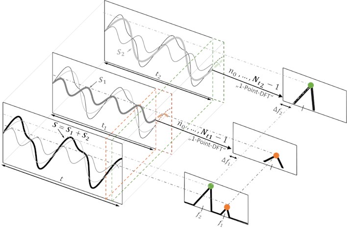
The window length is selected for every th frequency line in a manner that in the trimmed signals of are always -dependent integer periods (Fig. 2). In this way, the variable window length is a function of and depends therefore on the frequency.
Fig. 2Schematic diagram of the Trimmed Window Discrete Fourier Transform (TWDFT) approach
Subsequently, the DFT algorithm is applied on a frequency-dependent sample number . In Eq. (3-10) the derivation of is described. First, the existing frequency-dependent number of periods is determined:
where is the sampling time – this is the time between the acquisition of two samples. In the following step, the number of integer periods of the corresponding frequency is determined by rounding (Gaussian brackets):
The frequency-dependent signal duration is derived by dividing the number of integer periods by the corresponding frequency:
The theoretical number of samples associated with is determined by dividing by the sampling time as follows:
Since the can only be a positive integer, is determined by rounding :
The calculation of for integer periods is not sufficient to calculate an exact amplitude for the fractional frequency= 4.2 Hz from the example in Fig. 1. However, in order to be able to perform an evaluation between two spectral lines, the domain of has to be increased according to Eq. (2). Therefore, if the desired frequency resolution is known, the domain of is as follows:
where is the index of the frequency. Then the frequency results in:
The additional term in Eq. (9) indicates that the signal cannot contain whole periods of frequencies smaller than Hz. For example, a signal with a duration of = 1 s will not contain a whole period of a signal component with a frequency< 1 Hz.
With respect of Eq. (7) and Eq. (9), the calculation of is as follows:
Fig. 3Section of the frequency-dependent sample number Nf from a signal with 280 samples and a desired frequency resolution of ∆fdes = 0.01 Hz
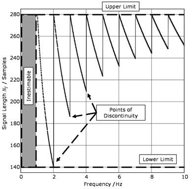
Fig. 3 showsfrom a signal with = 280 Hz and = 280 like the blue signal from Fig. 1(a) with a desired frequency resolution of = 0.01 Hz. In order to calculate an adjusted signal length, also for fractional frequencies according to Eq. (10), is set to 0.01 Hz. It can be seen that for integer frequencies (e.g. 1 Hz, 2 Hz, etc.) the complete sample number (= 280, “Upper Limit”) is always used since these frequencies are already represented in the signal by integer periods. For fractional frequencies, the sample number is trimmed down to = 140 as the “Lower Limit”, so that the signal is available as a whole-period signal corresponding to a specific frequency. The lower frequency limit can be determined according to Eq. (1), because no frequency can be estimated below it. The upper frequency limit is predefined according to the sampling theorem – for frequencies near the upper frequency limit, is close to The “Points of Discontinuity” are therefore discussed in more detail in subsection 2.3.
2.2. Substitution of the continuous frequency
To calculate the discrete Fourier spectrum of a sampled signal , the Fourier spectrum is approximated by neglecting the small terms according to Eq. (11), so that only frequency values are derived from sample:
For DFT calculation, only equidistant samples (where = 0,…, ) of the Fourier spectrum are determined in the interval . If the continuous variable in Eq. (11) is replaced by the discrete variable , the result is the usual expression for the DFT in Eq. (2) [33]. By an exponent comparison of Eq. (11) and Eq. (2), it can be seen that:
Solving Eq. (12) for leads to:
where is frequency-dependent and becomes:
Therefore, the original variable in the exponent of the Euler formula differs from the variable in the TWDFT approach. Accordingly, the complete expression for the TWDFT is given in Eq. (15), with respect to Eq. (2), (9), (10) and (14):
2.3. Special features
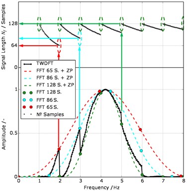
In the following section the points of discontinuity in Fig. 3 are discussed in more detail and their consequences for the amplitude spectrum are analysed. For this purpose, the blue simulated signal from Fig. 1 is considered again. For reasons of visualization, is set to 180 Hz. The signal duration remains at one second. The input vector of the DFT or FFT algorithm for calculating the spectral amplitude has the same length for each frequency line. In the TWDFT approach (Fig. 4(a)), the number of samples is different for each frequency. The discontinuities in the number of samples result in lateral peaks to the main lobe in the spectrum.
In Fig. 4(a), there are six further amplitude spectra shown depending on the FFT algorithm. The difference between the three dotted spectra is the length of the input vectors. Thereby, the more the original signal is shortened, the greater the main lobe width of the signal frequency = 4.2 Hz. For the three dashed spectra, the original signal is padded with zeros until the length of the input vector of 1024 samples is filled to interpolate the signal spectrum without adding any additional spectral information [33].
In Fig. 4(a), the amplitudes of the lateral peaks have short input vectors (red and cyan arrows). These amplitude values are based on the corresponding FFT spectra having the same length of the input vectors. The drop of the amplitude values of the TWDFT spectrum beside the frequency = 4.2 Hz and the length of its input vectors complies with the full sample number. These amplitude values also correspond to the green FFT spectrum. In this example, the red spectrum indicates the upper limit of the amplitude height. The green spectrum marks the lower limit of the amplitude spectrum. This means that the TWDFT amplitude spectrum is a kind of locus. Thereby the lateral peaks never reach the main lobe. For higher frequencies, the lateral peaks are smaller, because of smaller differences in the sample numbers at the discontinuities (Fig. 4(b)).
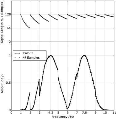
Fig. 4a) Relationship between the variable window length Nf and the lateral peaks beside the frequency f = 4.2 Hz; b) influence of the variable window length on two neighbouring frequencies (f1 = 4.2 Hz, f2 = 7.8 Hz) of a multi-frequency signal
a)
b)
Fig. 4(b) illustrates the amplitude spectrum based on TWDFT of a multi-frequency signal with two neighbouring frequencies (= 4.2 Hz, = 7.8 Hz). Both frequencies are calculated with sufficient accuracy. Nevertheless, it should be mentioned that the distance between two neighbouring frequencies has a limit according to Eq. (1). The influence of the variable window length on this distance has be taken into account.
3. Simulative study
In this chapter, the proposed estimator is compared to state of the art estimators in different scenarios. Within this simulation study, always the same real and noisy mono-frequency sinusoidal signal is used. Its mathematical description is given by Eq. (16). To verify the robustness of the parameter estimation under realistic conditions, an additive white Gaussian noise (AWGN) is added to the signal. The technical quality of the noisy signal is expressed by the signal-to-noise ratio (SNR):
The calculation of SNR in decibels is as follows:
Eq. (16) and Eq. (17) have the following properties:
– Signal amplitude as a function of SNR
– Variable SNR, where the effective value of the noise remains constant and the effective value of the signal increases continuously
– Signal frequency = 4.22 Hz
– = 280 with = 0,…,, = 280 Hz
– AWGN respectively with = 1
At the beginning of the article, it is described that the proposed approach is suitable for multi-frequency signals. At this point, it is decided to use a mono-frequency simulation signal, because this estimation approach is also applicable for mono-frequency signals. Furthermore, the automated evaluation of spectra has to be kept simple by using an easily understandable example.
3.1. Windowing functions
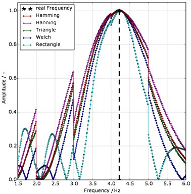
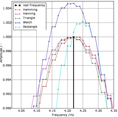
First, the influence of the window types (Hamming, Hanning, Triangle, Welch, Rectangle) on the estimation error of the TWDFT is investigated. The windowing itself is applied after the signal trimming and before the calculation of a complex spectral component at a certain frequency. For first considerations, the pure sinusoidal signals, without AWGN, are considered (Fig. 5).
Fig. 5Comparison between the 5 window functions used in the Trimmed Window Discrete Fourier Transform (TWDFT) approach; a) section of the amplitude spectra; b) detail view of the section
a)
b)
The comparison of the window types in Fig. 5(a) shows that the rectangular window has the narrowest main lobe and the largest side lobes. The frequency of = 4.22 Hz and the amplitude of = 1 is not exactly reached, but the discontinuities are relatively small. The Welch window has a narrow main lobe, low discontinuities and an acceptable frequency estimation. Nevertheless, a compromise has to be found because its amplitude is significantly higher than those of the others are. The results for the Hamming and Triangle windowing functions are almost identical.
To evaluate the estimation quality depending on the window type, the MSE is used:
The MSE indicates how much a point estimator spreads around the value to be estimated, where is the estimation, is the true value and n is the total population. Finally, the MSE is mapped as a function of the variable. Special attention is paid to the CRLB [3-6], [27, 28] and [34, 35]. It represents the lower limit for the MSE of estimators. The estimator is efficient if its MSE is smaller than the MSE of other estimators or if the MSE reaches the CRLB. Accordingly, the calculations of the CRLB for the estimated frequency and the estimated amplitude are given by Eqs. (19-20):
where:
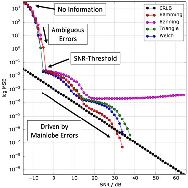
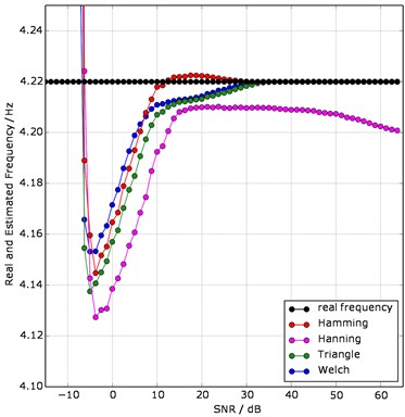
Fig. 6Frequency estimation a) Cramer-Rao lower bound (CRLB) and mean squared error (MSE); b) estimated and real frequency f = 4.22 Hz; both as a function of the signal-to-noise ratio in dB (SNRdB) of the window types
a)
b)
Fig. 6 illustrates the influence of the window functions on the estimation error. The desired frequency resolution of the TWDFT algorithm is = 0.01 Hz. For averaging the estimated noisy frequency values, the total population is= 20,000 (values per data point in Fig. 6). The logarithmic MSE depending on the with respect to Eq. (18).
In Fig. 6(b) the real frequency and the estimated frequency are shown as a function of the . In the upper range up to= –15 dB no information for an estimation is available. In this range, the interpretation is not possible because the effect of the noise on the amplitude spectrum is too strong. Noise and signal amplitudes lead to an incorrect estimate between –15 dB and –6 dB. From –6 dB, an asymptotic behaviour is observed, where the errors of the main lobes are the main factors, caused by the influence of the estimators themselves [36].
The frequency estimator with the Hamming window already exceeds the CRLB at = 30 dB, which means that the estimated frequency matches the real frequency (= 0). For frequency estimation, the Hamming window has a better influence than the other window types as shown in Fig. 5(b). From approximately = 10 dB this estimator is very close to the signal frequency. Fig. 7 gives the influence of the window functions on the amplitude estimation. The CRLB is a horizontal line according to Eq. (20), since the noise amplitude is always kept constant.
Fig. 7Amplitude estimation a) Cramer-Rao lower bound (CRLB) and mean squared error (MSE); b) estimated and real amplitude; both as a function of the signal-to-noise ratio (SNR) of the four window functions
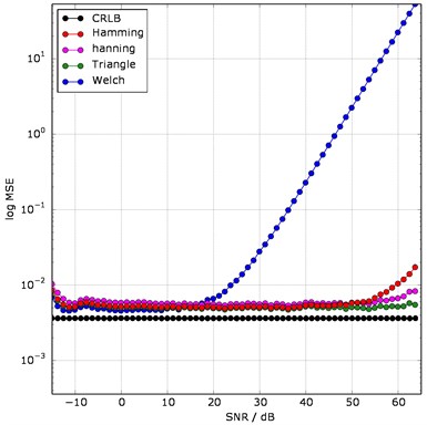
a)
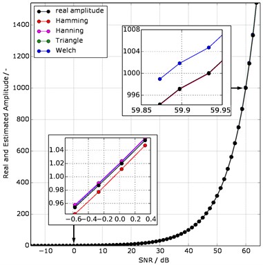
b)
As already shown in Fig. 5 and finally in Fig. 7(a), the Welch window has large errors in comparison to the other window functions. The increase of its MSE at = 20 dB results from the growing difference between the estimated and the real amplitude in Fig. 7(b). The Triangle window performs as the best among the compared windowing functions. In general, the better the leakage effect is suppressed, the better the amplitude is estimated. For the TWDFT algorithm, we will therefore adopt the Hamming window. It gives the best frequency estimation and has similar results for amplitude estimation to the Triangle window.
3.2. Comparison with state of the art estimators
To assess the MSE of the frequency and amplitude estimation of the TWDFT estimator, we compare it to established state of the art estimators. Fig. 8 shows the comparison by using the example data set from Eq. (16).
Comparing Fig. 1(b) to Fig. 8, the graphs “FFT” and “win FFT” remain unchanged. In contrast, “Spline win FFT” shows a good approximation to the real frequency and its amplitude. Nevertheless, the estimation results are not as good as those of the TWDFT estimator.
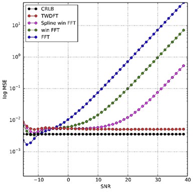
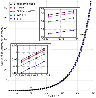
For the evaluation and comparison of the estimation error under the influence of noise, the MSE is displayed against the variable . For averaging the estimated noisy frequency values, is set to 20,000 values. Fig. 9(a) and (b) gives the frequency estimation and Fig. 10(a) and (b) shows the amplitude estimation.
Fig. 8Comparison of the four amplitude spectra of the sinusoidal signal without additive white Gaussian noise (AWGN); with detail view
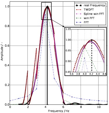
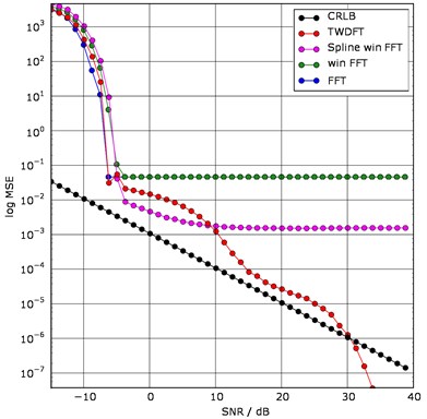
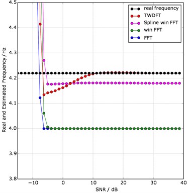
Fig. 9Frequency estimation a) Cramer-Rao lower bound (CRLB), mean squared error (MSE); b) the estimated and real frequency f = 4.22 Hz; both as a function of the signal-to-noise ratio (SNR) of the four estimators
a)
b)
“FFT” and “win FFT” have almost identical MSE values, due to the fixed frequency resolution = 1 Hz in the amplitude spectrum. Because the other two estimators offer a higher frequency resolution = 0.01 Hz, their values for the MSE are lower. Nevertheless, “TWDFT” achieves the real frequency value compared to “Spline win FFT” at lower noise. “Spline win FFT” do not achieve this and stagnates. To evaluate the error of the amplitude estimators, the MSE (Fig. 10(a)) and the real and estimated amplitudes (Fig. 10(b)) are examined as functions of the .
All estimators, with the exception of TWDFT, show high MSE values even at a small SNR (starting at –6 dB) resulting from large amplitude differences between the real and estimated amplitudes (Fig. 10(b)). The MSE of “TWDFT" remains low over all the considered SNR range.
The range before = –6 dB is unsuitable for evaluation, because the noise component in the spectrum is too high. Nevertheless, "FFT" shows a lower MSE as the CRLB, resulting from the addition of frequency and noise amplitudes, therefore the estimated amplitude is close to the real amplitude. The cause is that the AWGN covers all frequencies in the spectral range like an offset. At the windowed estimators “TWDFT”, “Spline win FFT” and “win FFT”, the sum of the frequency and noise amplitudes is too large to be below the CRLB, since the window always raises the main lobes, see Fig. 1(b). According to Eq. (18), this leads to a larger MSE.
From = –6 dB to the end of the range, it behaves similar to Fig. 7(a). The better the estimator eliminates the leakage effect, the better estimation results are achieved at a higher SNR.
Fig. 10Amplitude estimation a) Cramer-Rao lower bound (CRLB), mean squared error (MSE); b) estimated and real amplitude; both as a function of the signal-to-noise ratio (SNR) of the 4 estimators
a)
b)
4. Application to the vibration signal of a tram gearbox
In order to evaluate the performance of the novel frequency estimator, we apply it to real data acquired from vibrations of a tram gearbox. Vibration signals give information about gear meshing anomalies as well as the speed during operations to perform predictive maintenance. An accurate estimation of spectral components is therefore of a big interest.
4.1. Measurement dataset
The measurement dataset consists of the structure-borne sound (acceleration) and the motor speed (Fig. 11). The structure-borne sound was detected by an IEPE accelerometer of type KS80 in vertical measuring direction. The sensor was screwed in a gearbox housing borehole for an eyebolt near the gearbox output shaft. The measuring time is 10 seconds at a sampling rate of 51.2 kHz. The maximum tram speed is 50 km/h [2].
The gearbox has two stages, therefore it has two tooth mesh frequencies. By multiplying the motor speed (RPM) by the number of teeth (z1, z4), the theoretical courses of the first and second tooth mesh frequency is calculable. We use these calculations to evaluate the estimation results of the two spectrograms in Fig. 12.
4.2. Short-time TWDFT versus STFT
Short-time analyses of vibration signals offer a detailed spectral evaluation in the context of a time-frequency analysis. It provides information about the time dependence of frequency components of a vibration signal. In Fig. 12 short-time analyses based on the TWDFT-estimator and a STFT are compared and performed using the vibration signal from Fig. 11.
Fig. 11a) Vibration signal of a tram gearbox at a speed of 50 km/h, b) schematic of the gearbox structure and the measuring locations of the acceleration sensor (S) and the motor speed sensor (RPM)
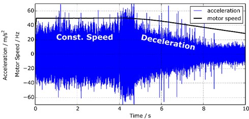
a)

b)
Fig. 12a) Time-frequency plot based on the Trimmed Window Discrete Fourier Transform (TWDFT) estimator, b) Time-frequency plot based on the STFT (single windows with FFT)
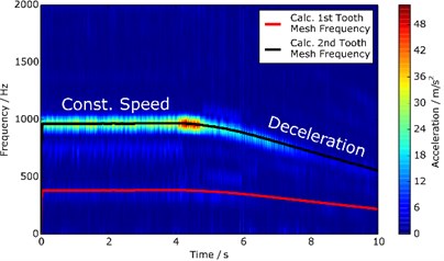
a)
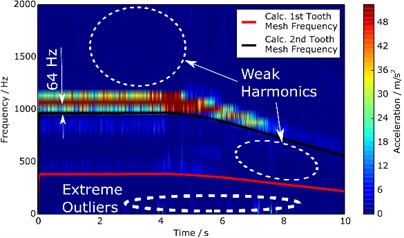
b)
Fig. 12 shows the time-frequency representation of the tram gearbox acceleration signal as a colour map. Fig. 12(b) is computed on the basis of a short-time Fourier Transform (STFT). Here the FFT algorithm is applied to single signal parts. Fig. 12(a) is computed on the basis of a short-time TWDFT (STTWDFT). The theoretical courses of the first and the second tooth mesh frequency (,) is calculated on the basis of the motor speed from Fig. 11. The comparison between the calculated und the FFT-based estimated tooth mesh frequencies shows impressively that the second tooth mesh frequency ( 968 Hz) in Fig. 12(b) is shifted further to the top side of the calculated tooth mesh frequency. This is because of the frequency resolution 64 Hz according to Eq. (1) and the associated stair-like appearance of the frequencies. Also the amplitudes of the harmonics of the first tooth mesh frequency ( 383 Hz) are much weaker than in Fig. 12(a). By analysing the signal sequence between the 8th and 10th second in Fig. 11, it can be seen that the frequencies in Fig. 12(a) do not disappear in the noise and the harmonics are better formed than in Fig. 12(b). Similarly, special operation processes of the gearbox can be detected, e.g. the start of the braking process, which results in higher contact forces and vibrations between the gears.
5. Conclusions
Frequency and amplitude estimation is particularly challenging for noisy signals that are present in short time intervals. In this contribution, we propose a novel estimator the TWDFT for aperiodic and multi-frequency noisy signals and compared it to classical estimators as well as with the Cramer-Rao lower bound (CRLB). The estimator is based on the DFT calculation, at one frequency-point followed by a segmentation of the input time domain signal in such a way, that its length is an integer number of periods corresponding to this frequency. The windowing of the signal by a Hamming window reached thereby the best estimation results.
The estimation error was evaluated by the mean squared error (MSE). A mono-frequency signal has been selected as simulation data set for the evaluation. To investigate the robustness of the estimator under the influence of noise, an additive white Gaussian noise (AWGN) was added to the signal. The MSE is mapped using the signal-to-noise ratio (SNR) from –15 dB to 40 dB.
Compared to other estimators, excellent results are obtained in spite of a big noise range. TWDFT estimates better than FFT from an SNR of –6 dB. At an SNR of 30 dB, the estimator reaches the real value of the frequency and at higher SNR values it falls under the CRLB. Applying the TWDFT estimator as a short-time analysis to a vibration signal of a tram gearbox shows that significantly more differentiated analyses of the frequency components over time can be performed in comparison to the short-time Fourier transform (STFT).
The realized estimator has therefore significant advantages considering its reduced sensitivity to signal noise and uses a relative short signal to reach a good quality of estimation. It is therefore especially suitable for application in embedded low-power systems for condition monitoring.
References
-
J. Shi, G. Du, R. Ding, and Z. Zhu, “Time frequency representation enhancement via frequency matching linear transform for bearing condition monitoring under variable speeds,” Applied Sciences, Vol. 9, No. 18, p. 3828, Sep. 2019, https://doi.org/10.3390/app9183828
-
M. Wolf, M. Rudolph, and O. Kanoun, “Concept for an event-triggered wireless sensor network for vibration-based diagnosis in trams,” Vibroengineering PROCEDIA, Vol. 27, pp. 55–60, Sep. 2019, https://doi.org/10.21595/vp.2019.21033
-
C. Candan, “Fine resolution frequency estimation from three DFT samples: Case of windowed data,” Signal Processing, Vol. 114, pp. 245–250, Sep. 2015, https://doi.org/10.1016/j.sigpro.2015.03.009
-
C. Candan, “Analysis and further improvement of fine resolution frequency estimation method from three DFT samples,” IEEE Signal Processing Letters, Vol. 20, No. 9, pp. 913–916, Sep. 2013, https://doi.org/10.1109/lsp.2013.2273616
-
K. Werner and F. Germain, “Sinusoidal parameter estimation using quadratic interpolation around power-scaled magnitude spectrum peaks,” Applied Sciences, Vol. 6, No. 10, p. 306, Oct. 2016, https://doi.org/10.3390/app6100306
-
M. D. Macleod, “Fast nearly ML estimation of the parameters of real or complex single tones or resolved multiple tones,” IEEE Transactions on Signal Processing, Vol. 46, No. 1, pp. 141–148, 1998, https://doi.org/10.1109/78.651200
-
X. Liu, Y. Ren, C. Chu, and W. Fang, “Accurate frequency estimation based on three-parameter sine-fitting with three FFT samples,” Metrology and Measurement Systems, Vol. 22, No. 3, pp. 403–416, Sep. 2015, https://doi.org/10.1515/mms-2015-0032
-
Hainsworth S. and Macleod M., “On sinusoidal parameter estimation,” in Proceedings of the 6th Conferenece on Digital Audio Effects (DAFx-03), 2003.
-
G. Bai, Y. Cheng, W. Tang, and R. Shi, “Accurate iterative frequency estimation by a new interpolator,” in 2018 10th International Conference on Wireless Communications and Signal Processing (WCSP), p. 2018, Oct. 2018, https://doi.org/10.1109/wcsp.2018.8555734
-
A. Serbes, “Fast and efficient sinusoidal frequency estimation by using the DFT coefficients,” IEEE Transactions on Communications, Vol. 67, No. 3, pp. 2333–2342, Mar. 2019, https://doi.org/10.1109/tcomm.2018.2886355
-
J. Borkowski, D. Kania, and J. Mroczka, “Comparison of sine-wave frequency estimation methods in respect of speed and accuracy for a few observed cycles distorted by noise and harmonics,” Metrology and Measurement Systems, Vol. 25, No. 2, pp. 283–302, 2018, https://doi.org/10.24425/119567
-
L. Fan, G. Qi, J. Xing, J. Jin, J. Liu, and Z. Wang, “Accurate frequency estimator of sinusoid based on interpolation of FFT and DTFT,” IEEE Access, Vol. 8, pp. 44373–44380, 2020, https://doi.org/10.1109/access.2020.2977978
-
G. Bai, Y. Cheng, W. Tang, S. Li, and X. Lu, “Accurate frequency estimation of a real sinusoid by three new interpolators,” IEEE Access, Vol. 7, pp. 91696–91702, 2019, https://doi.org/10.1109/access.2019.2927287
-
R. Diao and Q. Meng, “Frequency estimation by iterative interpolation based on leakage compensation,” Measurement, Vol. 59, pp. 44–50, Jan. 2015, https://doi.org/10.1016/j.measurement.2014.09.039
-
A. Serbes, “Fast and efficient estimation of frequencies,” IEEE Transactions on Communications, Vol. 69, No. 6, pp. 4054–4066, Jun. 2021, https://doi.org/10.1109/tcomm.2021.3067383
-
A. Serbes and K. Qaraqe, “A fast method for estimating frequencies of multiple sinusoidals,” IEEE Signal Processing Letters, Vol. 27, pp. 386–390, 2020, https://doi.org/10.1109/lsp.2020.2970837
-
Y. E. Garcia, P. Kovacs, and M. Huemer, “Variable projection for multiple frequency estimation,” in ICASSP 2020 – 2020 IEEE International Conference on Acoustics, Speech and Signal Processing (ICASSP), p. 2020, May 2020, https://doi.org/10.1109/icassp40776.2020.9052907
-
Y. E. G. Guzman, M. Lunglmayr, and M. Huemer, “A gradient ascent approach for multiple frequency estimation,” in Computer Aided Systems Theory – EUROCAST 2019, Cham: Springer International Publishing, 2020, pp. 20–27, https://doi.org/10.1007/978-3-030-45096-0_3
-
S. S. Abeysekera, “Least-squares multiple frequency estimation using recursive regression sum of squares,” in 2018 IEEE International Symposium on Circuits and Systems (ISCAS), pp. 1–5, May 2018, https://doi.org/10.1109/iscas.2018.8351138
-
S. Luo, F. Zhang, C. Liu, and R. Y. Zhong, “Frequencies estimation of gearbox vibration signal based on normalized lattice filter with RLS-based algorithm,” Measurement Science and Technology, Vol. 32, No. 1, p. 015104, Jan. 2021, https://doi.org/10.1088/1361-6501/aba93a
-
V. Popović-Bugarin and S. Djukanović, “A low complexity model order and frequency estimation of multiple 2-D complex sinusoids,” Digital Signal Processing, Vol. 104, p. 102794, Sep. 2020, https://doi.org/10.1016/j.dsp.2020.102794
-
P. Pan, Y. Zhang, Z. Deng, and W. Qi, “Deep learning-based 2-D frequency estimation of multiple sinusoidals,” IEEE Transactions on Neural Networks and Learning Systems, pp. 1–12, 2021, https://doi.org/10.1109/tnnls.2021.3070707
-
S. Djukanovic and V. Popovic-Bugarin, “Efficient and accurate detection and frequency estimation of multiple sinusoids,” IEEE Access, Vol. 7, pp. 1118–1125, 2019, https://doi.org/10.1109/access.2018.2886397
-
D. Kang, P. Chenghao, and L. Weihua, “Spectrumanalysis comparison between ZFFT and Chirp-Z Transform,” Journal of Vibration and Shock, Vol. 25, pp. 9–12, 2006.
-
D. Granados-Lieberman, R. Romero-Troncoso, E. Cabal-Yepez, R. Osornio-Rios, and L. Franco-Gasca, “A real-time smart sensor for high-resolution frequency estimation in power systems,” Sensors, Vol. 9, No. 9, pp. 7412–7429, Sep. 2009, https://doi.org/10.3390/s90907412
-
B. Al-Qudsi, N. Joram, A. Strobel, and F. Ellinger, “Zoom FFT for precise spectrum calculation in FMCW radar using FPGA,” in 2013 9th Conference on Ph.D. Research in Microelectronics and Electronics (PRIME), Jun. 2013, https://doi.org/10.1109/prime.2013.6603180
-
M. D. Ortigueira and C. J. C. Matos, “Fractional discrete-time signal processing: scale conversion and linear prediction,” Nonlinear Dynamics, Vol. 29, No. 1/4, pp. 173–190, 2002, https://doi.org/10.1023/a:1016522226184
-
M. D. Ortigueira, A. S. Serralheiro, and J. A. Tenreiro Machado, “A new zoom algorithm and its use in frequency estimation,” Waves, Wavelets and Fractals, Vol. 1, No. 1, pp. 17–21, Nov. 2015, https://doi.org/10.1515/wwfaa-2015-0002
-
F. Jing, C. Zhang, W. Si, Y. Wang, and S. Jiao, “Polynomial phase estimation based on adaptive short-time fourier transform,” Sensors, Vol. 18, No. 2, p. 568, Feb. 2018, https://doi.org/10.3390/s18020568
-
T. R. F. Mendonca, C. H. N. Martins, M. F. Pinto, and C. A. Duque, “Variable window length applied to a modified Hanning filter for optimal amplitude estimation of power systems signals,” in 2015 IEEE Power and Energy Society General Meeting, Jul. 2015, https://doi.org/10.1109/pesgm.2015.7285859
-
T. R. F. Mendonca, M. F. Pinto, and C. A. Duque, “Adjustable window for amplitude estimation considering the time-varying frequency of power systems signals,” in 2015 IEEE 24th International Symposium on Industrial Electronics (ISIE), Jun. 2015, https://doi.org/10.1109/isie.2015.7281665
-
D. Hart, D. Novosel, Yi Hu, B. Smith, and M. Egolf, “A new frequency tracking and phasor estimation algorithm for generator protection,” IEEE Transactions on Power Delivery, Vol. 12, No. 3, pp. 1064–1073, Jul. 1997, https://doi.org/10.1109/61.636849
-
Tan L. and Jiang J., Digital Signal Processing: Fundamentals and Applications. Third Edition, London: Academic Press, 2019, pp. 91–142.
-
D. Rife and R. Boorstyn, “Single tone parameter estimation from discrete-time observations,” IEEE Transactions on Information Theory, Vol. 20, No. 5, pp. 591–598, Sep. 1974, https://doi.org/10.1109/tit.1974.1055282
-
F. Rice, B. Cowley, B. Moran, and M. Rice, “Cramer-Rao lower bounds for QAM phase and frequency estimation,” IEEE Transactions on Communications, Vol. 49, No. 9, pp. 1582–1591, 2001, https://doi.org/10.1109/26.950345
-
C. D. Richmond, “Capon algorithm mean-squared error threshold SNR prediction and probability of resolution,” IEEE Transactions on Signal Processing, Vol. 53, No. 8, pp. 2748–2764, Aug. 2005, https://doi.org/10.1109/tsp.2005.850361
Cited by
About this article

