A versatile algorithm for estimating natural frequencies with high accuracy

1. Introduction

Features extracted from the vibration response are used since decades to characterize structures [1-3]. One of the main beneficiaries of structural identification is the field of non-destructive detection techniques. Currently, there are numerous methods for detecting defects based on vibration measurement [4-8]. The most common modal parameter used to detect defects is the natural frequency, because it can be easily measured and involves the use of simple and robust equipment. The mathematical relationship between the damage dimensions and the frequency drop is proposed in [9]. Because the damage has a low influence on the frequency changes, in order to observe the occurrence of damage as soon as possible [10], accurate frequency estimation is requested. The simplest way to achieve this target is using an interpolation method based on two spectral lines [11-13] or three spectral lines [14-16], but the results have been proved to be unsatisfactory for detecting damage in the early stage [17].

In prior research, we have developed several techniques to improve the frequency readability [18-20]. In our latest research, we have developed a structure excitation procedure that provides the highest amplitude for the targeted vibration mode [21]. In this paper, we complete the procedure with an original algorithm based on quadratic polynomial interpolation that helps finding the real frequency at an inter-line position. The novelty of the algorithm consists in applying the interpolation to spectral lines belonging to three different spectra obtained by stepwise shortening the acquired signal and finding the abscissa of the maximum obtained from the contrived polynomial function. The algorithm is implemented in Python as an application (PyFEST) and we tested its functionality for a signal containing three harmonics with known frequencies and amplitudes. We managed to estimate both frequencies and amplitudes with high accuracy and found that the application is easy to use and versatile, allowing the user to choose the optimal input parameters during the frequency evaluation process.

2. The proposed algorithm and its implementation in Python

The main disadvantage of estimating the natural frequencies for non-destructive testing by standard algorithms based on the Fourier transforms is the short length of the acquired signals, which results in a raw frequency resolution $\mathrm{\Delta }f$. While this resolution is somehow controllable for the Discrete Fourier Transform (DFT) but for the Fast Fourier Transform (FFT) it isn’t because the length of the analyzed signal depends on the specific number of samples that must be a power of 2. In consequence, the real frequency is typically located at a spectral inter-line position, and therefore an accurate estimation is not possible.

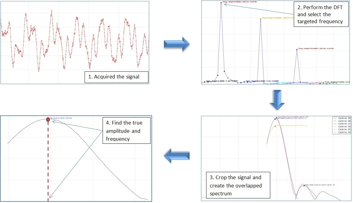
To overcome this inconvenient, we developed an algorithm which performs a quadratic interpolation based on three points that belong to three spectra, each spectrum being obtained for the original signal with a different time length. To be convinced that we have chosen the right points for interpolation, we execute a signal truncation until it is shortened to the length corresponding to two periods $T$ of the target frequency $f$. At each step, two samples are extracted from the signal, resulting in a large number of truncations for each $T$. In this way we obtain numerous amplitudes associated with the corresponding frequencies, which usually form three distinct curves: the first is a portion of a cycle, the second represents a whole cycle and the last again a portion of a cycle. Finally, we extract three points from the curve with the biggest amplitude which has a maximum and two neighbors and perform the interpolation. The achieved maximum of the polynomial represent the amplitude and its associated abscissa the real frequency. We implemented the algorithm in Python and a simple-to-use application resulted. The actions performed to run the program are presented in Table 1, along with the displayed results.

In the first step, the user select a CSV (preferably due to the increased data import speed) or Excel file containing the analyzed signal. The signal is displayed as shown in in Fig. 1.

Fig. 1The signal to be analyzed and the box for choosing the upper frequency limit to be analyzed

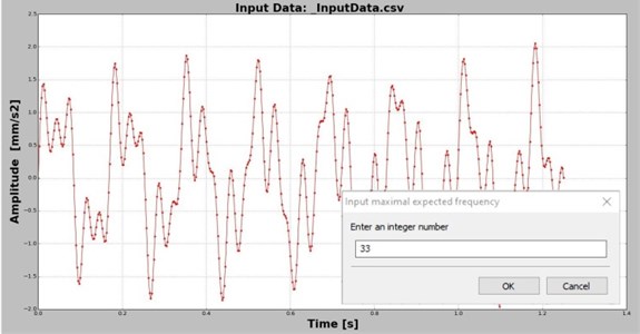
Along with the original signal representing the acquired or generated data, a box that permits the user to select the upper frequency limit is displayed in the center of the diagram. The frequency selected here will define the number of spectral lines for which the DFT is calculated. This option is available to save computing time, because the highest frequency $f_{Ny}$ found in the DFT is the half of the total number of samples $N$, and usually much bigger than the biggest frequency $f_{max}$ which is targeted in the analysis.

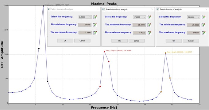
For the selected $f_{max}$ the DFT is calculated and plotted as shown in Fig. 2. In the plot area boxes indicating the frequencies that are local maxima ($f_1$, $f_2$ and $f_3$ in this case) and the frequencies for the neighbor spectral lines are displayed. Here, the user can select a frequency to be analyzed.

Fig. 2DFT obtained for the imported signal and boxes indicating the frequencies that are local maxima and their neighbors

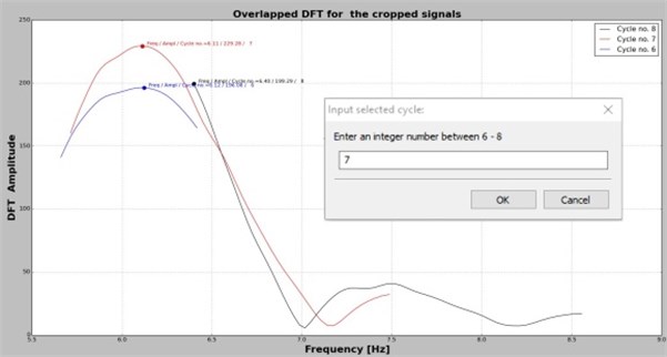
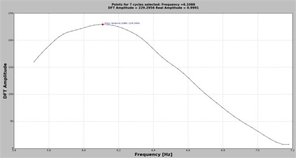
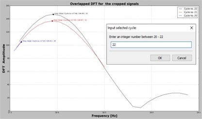
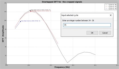
By selecting a frequency, let’s say $f_1$, the application perform DFT for the signal containing the original number of samples $N$. Afterward, two samples are cut consecutively from the signal until the original signal is shortened with $2T_1=2/f_1$ seconds. For all achieved signals the DFT is performed again and the biggest amplitude is plotted in a new graph, see Fig. 3(a), 3(c) and 3(e). The points are grouped in function of the cycle/period to which they belong. This information is displayed on the upper-right corner of the plot area. Note that, the DFT values are calculated just for the spectral lines that belong to the frequency domain framed by the neighbors of the targeted frequency $f_1$, again to save computing effort.

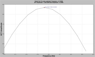
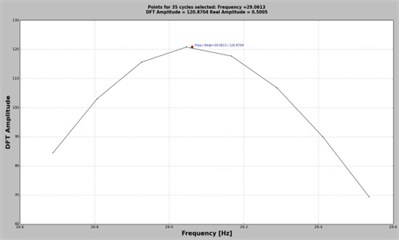
The user can select the proper number of cycles in the box located in the middle of the plot area. The implicit value is the median value found for the number of cycles that is 7 for the presented case in which $f_1$ is targeted. By selecting one of the suggested values, the application sorts all points belonging to the given cycle (Fig. 3(b)) and selects the maximizer and its two neighbors, which are used for interpolation. The polynomial function is found and its maximum is calculated. This maximum represents the DFT amplitude and its abscissa the real frequency. In order to find the real amplitude, the application divides the DFT amplitude by $N/2$. All three features, the real frequency, DFT amplitude and real amplitude are indicated at the top of the plot area in Fig. 3(b), 3(d) and 3(f).

For the frequency estimation process is crucial to select the right number of cycles. In order to obtain reliable points for interpolation, it is extremely important to achieve at least eight truncated signals, and consequently eight maximizer, that belong to one cycle/period. Also, the number of cycles contained in the original signal should be five, but preferably bigger than ten.

The estimation process must be repeated for all targeted frequencies; to this aim, steps 1 to 4 should be resumed.

Fig. 3The overlapped DFT in the selected frequency rage and the sorted values for the chosen cycle

a)

b)

c)

d)

e)

f)

3. Results and discussion

The first test concerns harmonic signals with the frequencies indicated in Table 2. All signals have the amplitude $A=$1 mm/s², and are generated with $N=$ 501 samples and have a time length $t=$1.25 seconds. The selected parameters, the estimated frequencies and the estimation errors are also presented in Table 2. It can be observed that the errors obtained by involving the Python application based on the original frequency estimation algorithm lead to excellent results, the errors being less than ±0,2 %, and in absolute values the frequencies estimated with this application are much closer than those obtained from a standard DFT.

A second approach considers a test signal composed of three harmonics with the frequencies and amplitudes indicated in Table 3. This signal simulates the first three modes of vibration of a beam. It is generated with $N=$ 501 samples and again has a length of time $t=$ 1.25 seconds.

The first harmonic component intentionally coincides with the first sinusoidal signal tested because we intended to see if the estimated frequencies in the composed signals are affected by the other harmonics. Analyzing the results in Tables 2 and 3 we observe that the frequency of 6.12 Hz is precisely identified, even if there is a very small difference between the results obtained for the simple signal and the one composed of three harmonics.

The frequencies of the other two components are also accurately estimated, which proves that the algorithm can be used with confidence in identifying the natural frequencies of beams and plates in mechanical or civil structures.

4. Conclusions

The proposed algorithm for estimating the natural frequencies of structures, for which we have designed the PyFEST application in Python, allows an accurate estimation of the natural frequencies of beams or plates. This application makes possible early assessment of cracks when using the vibration-based detection methods. We tested the application for signals composed by single or multiple harmonics with known frequencies and found that in all cases the frequencies and amplitudes are estimated with high accuracy, the errors being less than ±0.22 %. In fact, the frequencies can be read with an error occurred by the second digit after the dot even for high frequencies, which makes PyFEST extremely reliable.

We also found that, if the signal contains more harmonic components the energy of these components is easily spread along the spectrum (the so-called noise) and may slightly affect the precision of the estimation. By increasing the signal length this effect is diminished.