Study on fluctuating wind force and fluctuating wind pressure of heliostats

1. Introduction

The advancement and deployment of solar energy technologies are increasingly pivotal in shaping the trajectory of renewable energy innovation. The International Energy Agency (IEA) projects that solar power generation will constitute over 20 % of global electricity supply by 2040 [1]. Among solar thermal power generation technologies, tower-based systems exhibit the lowest levelized cost of energy (LCOE) [2, 3]. The heliostat field, as the core optical subsystem of these plants, constitutes a significant capital expenditure due to its large spatial footprint and high component density [4, 5]. Given their susceptibility to aerodynamic loading and proneness to wind-induced failure modes, heliostat wind resistance design necessitates multi-disciplinary analysis incorporating geometric, material, and environmental parameters [6-10]. Therefore, it is of great significance to be studied the problems of heliostat under wind load. Wind engineering studies on heliostat systems have undergone exponential growth, encompassing advanced numerical simulations, field measurements, and full-scale experimental investigations across multiple operational scenarios [11-17].

The author summarized the relevant researches on the force and wind pressure of heliostat, it is found that the pulsating wind force and pulsating wind pressure of heliostats are quite different from those of isolated heliostat due to the occlusion effect of heliostats. However, the achievements of heliostats are few and there is a lack of in-depth research. Given the prevalence of rectangular monolithic column support configurations in commercial heliostat deployments, this study undertakes a comprehensive aerodynamic characterization of this dominant structural typology [5]. By conducting wind tunnel test of wind force and wind pressure on the rigid model of heliostat, the variation law of pulsating wind force and pulsating wind pressure of heliostats is studied, and the corresponding working conditions and mirror surface positions of the maximum pulsating wind force and pulsating wind pressure are obtained. This study contributes to the aerodynamic characterization of heliostats by addressing critical knowledge gaps in previous investigations. The derived force-pressure relationships provide a foundational framework for advanced wind-resistant design methodologies.

2. Overview of the wind tunnel test

2.1. Equipment

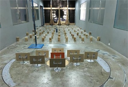
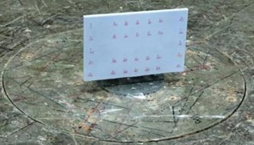
Wind tunnel experiments were conducted at Hunan University’s HD-3 atmospheric boundary layer wind tunnel facility using a scaled prototype of a northwest China tower solar thermal power station heliostat [1]. The Cobra probe anemometry system was employed to characterize the three-dimensional turbulent flow field, with detailed test configurations illustrated in Fig. 1.

Fig. 1Wind tunnel test of heliostats

The force measuring system is used a six-component force balance (Fig. 2). The force balance can be decomposed the wind force acting on the heliostat into the force components along the $X$, $Y$ and $Z$ axes and the torque components around the $X$, $Y$ and $Z$ axes which is according to the rectangular coordinate system (Fig. 3).

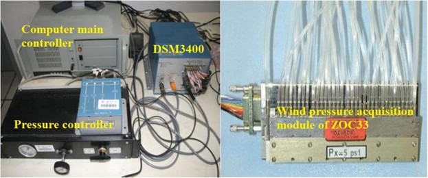
The pressure measurement system consists of a host computer, pressure regulator, and DSM3400 electronic pressure scanning valve (Fig. 4) for hardware components, complemented by custom signal acquisition and processing software operating at a 312.5 Hz sampling frequency.

Fig. 2Force balance

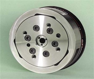
Fig. 3Force balance axis

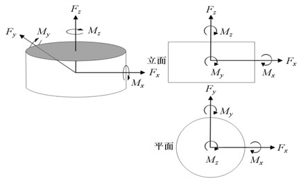
Fig. 4Pressure measuring system

2.2. Model and measurement point

The experimental model was constructed to a geometric scaling factor of 1:30 (Fig. 5), the dimensions of each part are shown in Table 1.

Table 1Dimensions of heliostat model components (Unit: mm)

Component	Length of mirror panel	Width of mirror panel	Height of strut	Length of rotating shaft	Length of support arms	Length of support plate	Width of support plate
Dimension	245	183	111	140	30	100	30

Fig. 5The front and back of the heliostat model

a) Front

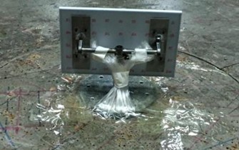
b) Back

Based on Gong et al.’s validation study [18], the mirror surface’ s gap size effects between mirror segments were deemed negligible for wind tunnel testing. Consequently, the heliostat model adopted a monolithic panel with 35 sub-mirrors to maintain geometric fidelity while simplifying the experimental setup. The double-sided symmetrical layout is used, and A total of 64 pressure transducers were distributed across both the front and rear surfaces of the heliostat mirror to capture high-resolution aerodynamic loading data. The arrangement of pressure taps is shown in Fig. 6.

Fig. 6pressure tap number and sub-mirror number

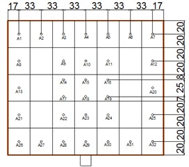
a) Front

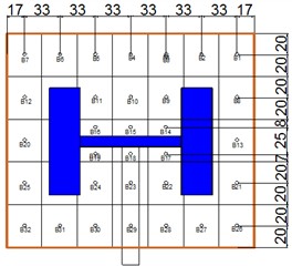
b) Back

c) Sub-mirror

2.3. Arrangement of heliostats

Radial grid configurations are preponderantly utilized in heliostat field layout optimization [19] (Fig. 7). This arrangement has certain advantages and this arrangement is reduced the occlusion effect between specular reflections. It is considering that the number of radial and circumferential heliostats are so many, only 9 heliostats in radial and circumferential five rows are selected for consideration.

Fig. 7Radial grid distribution

2.5. Test working conditions

The experimental campaign comprised 130 working conditions, each defined by a distinct combination of azimuth ($\beta$) and elevation ($\alpha$) angles. Azimuth angles were systematically varied at 15° intervals from 0° (windward) to 180° (leeward) in the anti-clockwise direction, while elevation angles were incremented at 10° steps from 0° (horizontal) to 90° (vertical). The coordinate system adopted for angular definitions is detailed in Fig. 10.

Fig. 8Wind speed profile and turbulence intensity profile

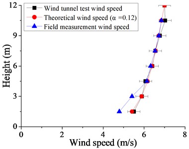
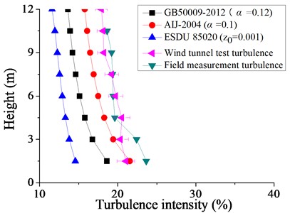
Fig. 9Downwind fluctuating wind speed power spectrum

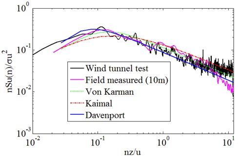
Fig. 10The coordinate system of wind tunnel test

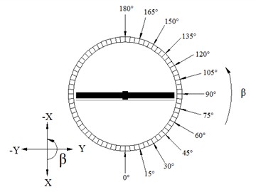
a) The coordinate system of azimuth angle $\beta$

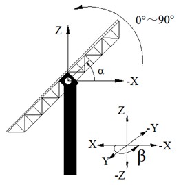
b) The coordinate system of elevation angle $\alpha$

2.6. Definition of parameters

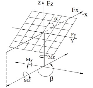
The force and moment coefficients of the heliostat are schematically defined in Fig. 11. The mathematical expressions for fluctuating force coefficients are provided below [21]:

1

$C_{Fx,fluc}=\frac{{\sigma }_{Fx}}{q_{H}A},$

2

$C_{Fy,fluc}=\frac{{\sigma }_{Fy}}{q_{H}A},$

3

$C_{Fz,fluc}=\frac{{\sigma }_{Fz}}{q_{H}A},$

4

$C_{Mx,fluc}=\frac{{\sigma }_{Mx}}{q_{H}AH},$

5

$C_{My,fluc}=\frac{{\sigma }_{My}}{q_{H}AH},$

6

$C_{Mz,fluc}=\frac{{\sigma }_{Mz}}{q_{H}AL},$

where ${\sigma }_{F_x}$, ${\sigma }_{F_y}$and ${\sigma }_{F_z}$denote the root mean square (RMS) values of the base shear forces in the $x$-, $y$-, and $z$-directions respectively. Similarly, ${\sigma }_{M_x}$, ${\sigma }_{M_y}$ and ${\sigma }_{M_z}$ represent the RMS amplitudes of the lateral, base overturning, and azimuth moment. $q_H$ denotes the reference wind velocity pressure, $q_H=1/2\rho \cdot V_H^2$. In the formula, $H=$ 0.111 m, which is represent the elevation axis height (hinge), $V_H$ is the mean wind speed at height $H$ during the testing, and $\rho$ is the air density. $A$ is the characteristic area (heliostat model mirror panel area). $L$ is the characteristic length (heliostat model mirror panel width).

Fig. 11The direction of force coefficients CF and moment coefficients CM for heliostat configurations

In structural wind engineering, the dimensionless wind pressure coefficient $C_P$ serves as a normalized metric to characterize aerodynamic loading on structural surfaces. For heliostat systems, this coefficient is specifically defined as the net differential pressure coefficient $C_{Pi}$ across the mirror panel, with its mathematical formulation provided in Eq. (7).

7

$C_{pi}\left(t\right)=\frac{P_i^f\left(t\right)-P_i^b\left(t\right)}{\frac{1}{2\rho V_H^2}},$

where $C_{Pi}$ represents the dimensionless pressure coefficient at the, $i$-th pressure tap, $P_i^f\left(t\right)$ and $P_i^b\left(t\right)$ denote the windward and leeward pressures at tap $i$. $\rho$ is air density, $V_H$ is the velocity at reference height $H=$ 0.4 m (prototype equivalent height: 12 m). A total of 10,000 samples per tap were collected at 312.5 Hz over 32 seconds, enabling calculation of mean and fluctuating $C_{Pi}$ using Eqs. (8-9):

8

$C_{pi,mean}=\frac{1}{N}{\sum }_{i=1}^N{C}_{pi}\left(t\right),$

9

$C_{pi,rms}=\sqrt{\frac{1}{N-1}{\sum }_{i=1}^N{\left(C_{pi}\left(t\right)-C_{pi,mean}\right)}^2},$

where $C_{Pi,mean}$ denotes the time-averaged pressure coefficient at tap $i$, $C_{Pi,rms}$ represents the root-mean-square (RMS) fluctuating component, and $C_{Pi}$ signifies the instantaneous time-series data. The indices $i$ = 1, 2,…, $N$ correspond to individual pressure taps, with $N$ denoting the total number of measurement locations.

3. Study on the fluctuating wind force of heliostats

Fig. 12 to Fig. 17 is shown the contour map and three-dimensional distribution map of fluctuating wind coefficient of heliostats under 130 working conditions, respectively.

Fig. 12Fluctuating and mean drag force coefficient

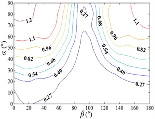
a) Distribution map of contour of $C_{Fx,fluc}$

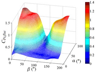
b) 3D distribution map of $C_{Fx,fluc}$

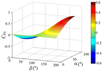
c) 3D distribution map of $C_{Fx}$

The fluctuating drag force coefficient is increased gradually from the bottom to the upper left and upper right corners of the distribution diagram. $C_{Fx,fluc}$ is reached the maximum value at working condition 0-90 and 180-90, and $C_{Fx,fluc}$is tended to the minimum value when $\beta =$ 90°. When $\beta =$ 90°, the heliostat mirror surface is parallel to the incoming wind and the load which is acting on the mirror surface is small, so $C_{Fx,fluc}$is small. As the change of angle, the mirror area which is perpendicular to the incoming wind is increased gradually, and the load which is acting on the mirror surface is also increased gradually, then $C_{Fx,fluc}$is increased gradually. When the working conditions are 0-90 and 180-90, the mirrors are perpendicular to the incoming wind, and the loads which are acting on the mirror are the largest on the working conditions. Therefore, the peak value of the fluctuating drag coefficient $C_{Fx,fluc}$ is found to be 1.371, and the corresponding working condition is 0-90. The 3D diagram of $C_{Fx,fluc}$ and $C_{Fx}$ can be compared, values of $C_{Fx,fluc}$ are both positive, if negative values in the 3D diagram of $C_{Fx}$ are taken as absolute values, the shape of the 3D diagram of the changed $C_{Fx}$ and $C_{Fx,fluc}$ is relatively similar. It is shown that the influence of incoming wind on $C_{Fx}$ and $C_{Fx,fluc}$ is consistent.

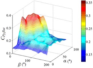
In the range of $\beta =$ 0°-75° and $\alpha =$ 30°-90°, values of $C_{Fy,fluc}$ are greater than 0.2, the change of values are obvious, and the distribution is like a mountain peak shape. In other working conditions, value of $C_{Fy,fluc}$are less than 0.2, the change of values are small, and the distribution is like a plane shape. Peak value of fluctuating lateral force coefficient $C_{Fy,fluc}$ is found to be 0.349, and corresponding working condition is 15-30. The 3D diagram of $C_{Fy,fluc}$ is similar to $C_{Fy,peak}$ of isolated heliostat, only the value is different. So, it is necessary to pay attention to the study of $C_{Fy,peak}$ and $C_{Fy,fluc}$ in the range of $\beta =$0°-75° and $\alpha =$ 30°-90°.

Fig. 13Fluctuating lateral force coefficient

a) Distribution map of contour of $C_{Fy,fluc}$

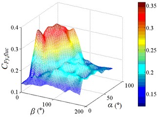
b) 3D distribution map of $C_{Fy,fluc}$

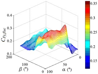
c) 3D distribution map of $C_{Fy}$

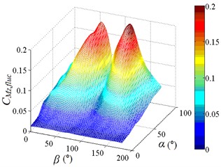
Fig. 14Fluctuating and mean lift force coefficient

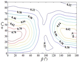
a) Distribution map of contour of $C_{Fz,fluc}$

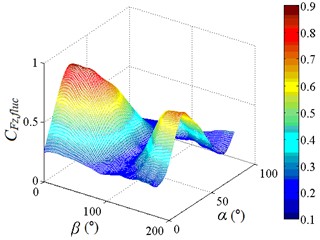
b) 3D distribution map of $C_{Fz,fluc}$

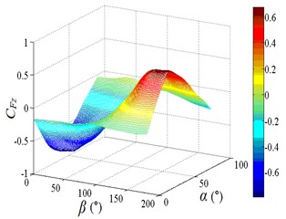
c) 3D distribution map of $C_{Fz}$

The fluctuating lift force coefficient is decreased at first and then increased with the increase of $\beta$, and the fluctuating lift force coefficient is increased at first and then decreased with the increase of $\alpha$. When $\beta =$ 90°-105°, values of $C_{Fz,fluc}$ are small. Peak value of the fluctuating lift force coefficient $C_{Fz,fluc}$ is found to be 0.858, and corresponding working condition is 0-30. The 3D diagram is distributed in two peaks on both sides with a trough in the middle. The 3D diagram of $C_{Fz,fluc}$ and $C_{Fz}$ can be compared, values of $C_{Fz,fluc}$ are both positive, if negative values in the 3D diagram of $C_{Fz}$ are taken as absolute values, the shape of the 3D diagram of the changed $C_{Fz}$ and $C_{Fz,fluc}$ is relatively similar. It is shown that the influence of incoming wind on $C_{Fz}$ and $C_{Fz,fluc}$ is consistent.

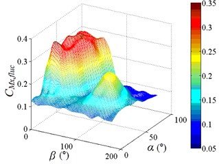
Fig. 15Fluctuating lateral moment coefficient and fluctuating lateral force coefficient

a) Distribution map of contour of $C_{Mx,fluc}$

b) 3D distribution map of $C_{Mx,fluc}$

c) 3D distribution map of $C_{Fy,fluc}$

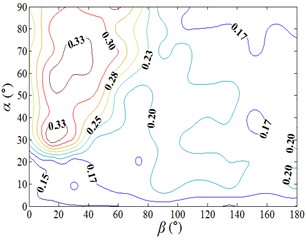
In the range of $\beta =$ 0°-75° and $\alpha =$ 30°-90°, values of $C_{Mx,fluc}$ are greater than 0.14, the change of values are obvious, and the distribution is like a mountain peak shape, and in the range of $\beta =$ 105°-150° and $\alpha =$ 20°-60°, the distribution is also like a mountain peak shape. In other working conditions, value of $C_{Mx,fluc}$are less than 0.14, the change of values are small, and the distribution is like a plane shape. Peak value of $C_{Mx,fluc}$ is found to be 0.334, and corresponding working condition is 15-30. The variation law of 3D diagram of $C_{Mx,fluc}$ is similar to the that of $C_{Fy,fluc}$, both of them are changed obviously in the range of $\beta =$ 0°-75° and $\alpha =$ 30°-90°, and the distribution are both like a mountain peak shape. The most difference is that changes of $C_{Mx,fluc}$ are also obvious in the range of $\beta =$ 105°-150° and $\alpha =$ 20°-60°, and the distribution is like a mountain peak shape, while changes of $C_{Fy,fluc}$ are little, and the distribution is like a plane shape. Therefore, it is necessary to pay attention to the study of $C_{Mx,fluc}$ in the range of $\beta =$0°-75° and $\alpha =$30°-90°.

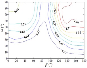
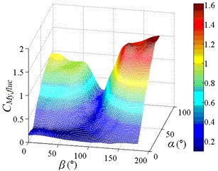
The distribution of $C_{My,fluc}$ is similar to that of $C_{Fx,fluc}$, $C_{My,fluc}$ is reached the maximum value when working condition 0-90 and 180-90, and $C_{My,fluc}$ is tended to the minimum value when $\beta =$ 90°. Peak value of $C_{My,fluc}$ is found to be 1.600, and corresponding working condition is 180-90. The 3D diagram of $C_{My,fluc}$ is similar to that of $C_{Fx,fluc}$, and the variation law is consistent.

Fig. 16Fluctuating base overturning moment coefficient and fluctuating drag force coefficient

a) Distribution map of contour of $C_{My,fluc}$

b) 3D distribution map of $C_{My,fluc}$

c) 3D distribution map of $C_{Fx,fluc}$

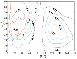
Fig. 17Fluctuating and mean azimuth moment coefficient

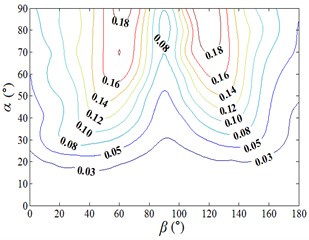
a) Distribution map of contour of $C_{Mz,fluc}$

b) 3D distribution map of $C_{Mz,fluc}$

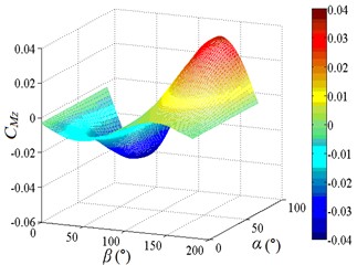
c) 3D distribution map of $C_{Mz}$

The fluctuating azimuth moment coefficient is increased at first and then decreased when $\beta =$ 0°-90° and $\beta =$ 90°-180°, and the fluctuating azimuth moment coefficient is increased with the increase of $\alpha$. Peak value of the fluctuating azimuth moment coefficient $C_{Mz,fluc}$ is found to be 0.199, and corresponding working condition is 135-90. The 3D diagram of $C_{Mz,fluc}$ and $C_{Mz}$ can be compared, values of $C_{Mz,fluc}$ are both positive, if negative values in the 3D diagram of $C_{Mz}$ are taken as absolute values, the shape of the 3D diagram of the changed $C_{Mz}$ and $C_{Mz,fluc}$ is relatively similar. It is shown that the influence of incoming wind on $C_{Mz}$ and $C_{Mz,fluc}$ is consistent.

From Table 2, the working condition of peak value of $C_{Fx,fluc}$ and $C_{My,fluc}$ is 0-90 and symmetrical working condition 180-90 respectively. Moreover, the 3D diagram of $C_{My,fluc}$ is similar to that of $C_{Fx,fluc}$, and the variation law is consistent. Which is because $F_x$ and $M_y$ is acted in the same direction, and $M_y$ is the result of the product of $F_x$ and the height of column. It is indicated that $C_{Fx,fluc}$ and $C_{My,fluc}$ are essentially the same. The working condition of peak value of $C_{Fy,fluc}$, $C_{Fz,fluc}$ and $C_{Mx,fluc}$is consistent, and the 3D diagram of $C_{Fy,fluc}$ is also similar to that of $C_{Mx,fluc}$, which is also based on the essence of $C_{Fy,fluc}$ and $C_{Mx,fluc}$. The working condition of peak value of $C_{Fz,fluc}$ and $C_{Mz,fluc}$ is consistent with that of $C_{Fz}$ and $C_{Mz}$, it is indicated that the importance of studying the peak value of fluctuating wind force coefficient and the corresponding working condition. Therefore, the study and analysis of heliostats need to be considered the peak value of fluctuating wind force coefficient and the corresponding working condition.

4. Study on the fluctuating wind pressure of heliostats

4.1. Fluctuating wind pressure distribution

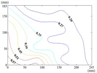
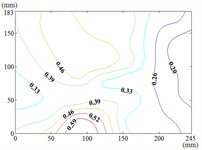
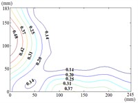
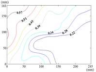
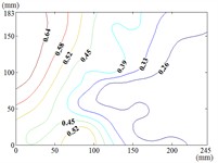
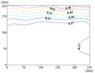
The heliostat’s actuation system enables continuous adjustment of both the azimuth ($\beta$) and elevation ($\alpha$) angles, necessitating systematic characterization of their combined effects on wind pressure distributions during wind-resistant design. Owing to spatial constraints, this study presents contour maps of fluctuating wind pressure coefficients under representative operational scenarios, as derived from wind tunnel testing.

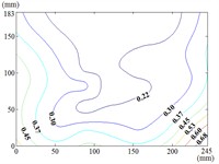
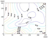
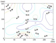
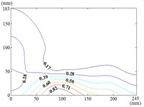
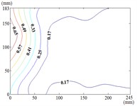
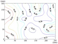
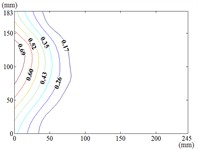
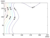
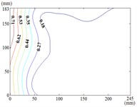
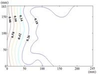
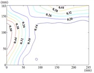
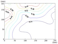
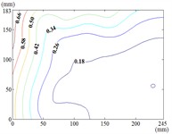
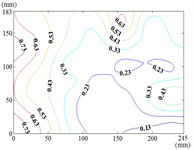
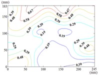
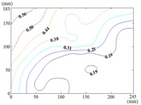
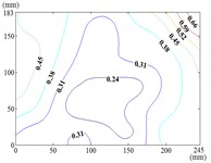
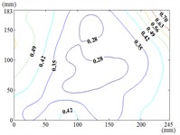
Fig. 18Fluctuating wind pressure coefficient

0-0

0-30

0-60

0-90

30-0

30-30

30-60

30-90

60-0

60-30

60-60

60-90

90-0

90-30

90-60

90-90

120-0

120-30

120-60

120-90

150-0

150-30

150-60

150-90

180-0

180-30

180-60

180-90

When the working condition 0-0, fluctuating wind pressure coefficient of heliostats is changed greatly in the lower 1/3 of the mirror surface, and which is gradually increased from top to bottom, and fluctuating wind pressure coefficient of heliostats is changed little in the upper 2/3 of the mirror surface. The interaction between the oncoming flow and the heliostat’s edge induces the formation of coherent cylindrical vortices, resulting in highly non-uniform fluctuating pressure distributions characterized by steep gradients at the windward boundary of the mirror surface. As the elevation angle $\alpha$ increases incrementally, the fluctuating wind pressure coefficient $C_{p,rms}$ exhibits a spatially evolving pattern, propagating radially outward from the centro-superior region to the mirror periphery. Maximum $C_{p,rms}$ values localize at the infero-right corner and left infero-marginal zone. At $\alpha =$90°, $C_{p,rms}$ gradients emanate symmetrically from the medio-superior edge, medio-dextral edge, and central mirror plane toward the lateral extremities.

When $\beta =$ 30° and $\alpha <$ 60°, the variation law of fluctuating wind pressure coefficients for heliostat arrays mirrors that of standalone heliostats, suggesting comparable coherent structures in the wake region. However, when $\alpha \ge$ 60°, the variation law of heliostats is changed, the peak value of the fluctuating wind pressure coefficient $C_{p,rms}$ localizes at the left-midpoint of the mirror's lower edge, with $C_{p,rms}$ attenuating progressively in the superior direction and then is gradually decreased to the right edge of the mirror when it is reduced to the middle of the mirror.

When $\beta =$ 60° and $\alpha <$ 90°, the variation law of fluctuating wind pressure coefficients for heliostat arrays mirrors that of standalone heliostats, indicating comparable coherent structures in the wake region. However, the fluctuating wind pressure coefficient of heliostats is varied greatly in the left 2/5 region of the mirror, the peak value of the fluctuating wind pressure coefficient $C_{p,rms}$ localizes at the left-midpoint of the mirror's lateral edge, with $C_{p,rms}$ attenuating progressively toward the right-hand side, and that of the remaining 3/5 region of the mirror is changed little. When $\alpha =$ 90°, Although the RMS pressure coefficient $C_{p,rms}$ attenuates progressively from the left edge to the right boundary, localized maxima emerge at the medio-dextral margin and infero-medial zone of the right edge, after which $C_{p,rms}$ continues its radial decay toward the mirror periphery.

When $\beta =$ 120° and $\beta =$ 150°, the variation law of fluctuating wind pressure coefficients for heliostat arrays mirrors that of standalone heliostats, except for the different sizes of the regions where the maximum and minimum values are distributed.

When working condition 180-0, the variation law of fluctuating wind pressure coefficients for heliostat arrays mirrors that of standalone heliostats, when $\beta =$ 180°, As the elevation angle α increases incrementally, the spatiotemporal migration of the minimum RMS pressure coefficient $C_{p,rms}$ zone shifts from the infero-mirror region to its central plane. This minimum zone exhibits a larger spatial extent compared to isolated heliostats due to wake interference effects. Concurrently, $C_{p,rms}$ undergoes anisotropic decay toward the uppero-left and uppero-right corners, culminating in a localized maximum at the uppero-dextral apex.

4.2. Maximum value of fluctuating wind pressure

Extreme values of the root-mean-square (RMS) fluctuating wind pressure coefficient $C_{p,rms}$, along with their corresponding working conditions, are tabulated in Tables 3 and 4 for both maximum and minimum conditions across the full test matrix.

Table 3Extreme values of the root-mean-square (RMS) fluctuating wind pressure coefficient Cp,rms across varying elevation angles α

$\alpha$	Maximum value of $C_{Pi,rms}$			Minimum value of $C_{Pi,rms}$
	$\beta$	Pressure tap	$C_{Pi,rms}$	$\beta$	Pressure tap	$C_{Pi,rms}$
0°	30°	A32	0.768	90°	A12	0.091
10°	90°	A8	0.702	120°	A19	0.089
20°	90°	A8	0.697	90°	A32	0.091
30°	180°	A7	0.672	90°	A32	0.088
40°	15°	A26	0.734	75°	A32	0.089
50°	60°	A8	0.628	75°	A12	0.087
60°	30°	A28	0.647	75°	A12	0.087
70°	30°	A28	0.677	75°	A12	0.088
80°	180°	A7	0.673	75°	A20	0.088
90°	120°	A8	0.729	75°	A12	0.096

For fixed elevation angles, the spatial distribution of peak RMS pressure coefficients $C_{p,rms}$ exhibits a relatively dispersed pattern, with maxima failing to cluster within specific wind incidence angles or pressure tap locations. Conversely, minimum $C_{p,rms}$values localize at 90° and 75° wind directions, corresponding to pressure taps A12 and A32. Table 3 documents the highest recorded $C_{p,rms}=$0.768 and the working condition is 30-0.

For fixed azimuth angles, the spatial distribution of peak RMS pressure coefficients $C_{p,rms}$ clusters at the uppero-marginal and infero-marginal zones of the mirror. Conversely, minimum $C_{p,rms}$ values localize at the dextral edges. Table 4 documents the highest recorded $C_{p,rms}=$0.768 and working condition is 30-0, consistent with the peak value and critical condition reported in Table 3. Collectively, Tables 3 and 4 reveal that $C_{p,rms}=$0.768 occurs at pressure tap A28, and working condition 30-0.

Table 4Extreme values of the root-mean-square (RMS) fluctuating wind pressure coefficient Cp,rms across varying azimuth angles β

$\beta$	Maximum value of $C_{Pi,rms}$			Minimum value of $C_{Pi,rms}$
	$\alpha$	Pressure tap	$C_{Pi,rms}$	$\alpha$	Pressure tap	$C_{Pi,rms}$
0°	0°	A28	0.625	10°	A4	0.103
15°	40°	A26	0.734	0°	A4	0.095
30°	0°	A28	0.768	0°	A4	0.092
45°	30°	A28	0.607	0°	A4	0.097
60°	90°	A8	0.679	80°	A12	0.091
75°	40°	A8	0.671	60°	A12	0.087
90°	10°	A8	0.702	30°	A32	0.088
105°	10°	A8	0.659	10°	A12	0.090
120°	90°	A8	0.729	10°	A19	0.089
135°	20°	A2	0.693	10°	A30	0.092
150°	0°	A5	0.717	10°	A30	0.100
165°	30°	A5	0.636	10°	A30	0.095
180°	80°	A7	0.673	0°	A30	0.101

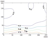
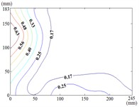
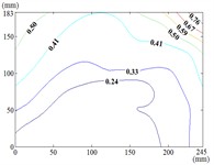
Fig. 19The contour maps of root-mean-square (RMS) fluctuating wind pressure coefficients Cp,rms under the most unfavorable working for heliostat configurations

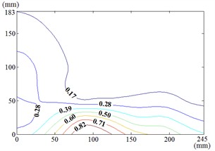
Fig. 19 is illustrated that under the working condition 30-0, the peak RMS pressure coefficient $C_{p,rms}$ localizes at the left-midpoint of the mirror’s lower edge, coinciding with the region where incident flow first interacts with the mirror surface. $C_{p,rms}$ attenuates progressively in the superior direction. The spatial location of the maximum mean pressure coefficient $C_p$ aligns precisely with that of $C_{p,rms}$. Therefore, the wind pressure resistance performance and related parameters of the mirror at this position should be analyzed and studied during the design of the heliostats.

4.3. Variation law of fluctuating wind pressure

4.3.1. Variation law of fluctuating wind pressure with azimuth angle

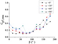
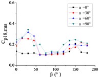
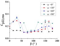
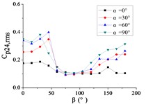
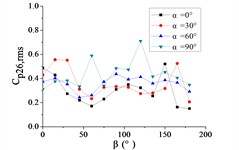
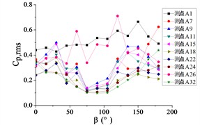
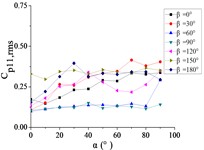
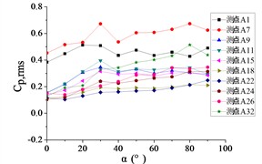
To systematically investigate the azimuthal angle’s effect on the RMS pressure coefficient $C_{p,rms}$ across distinct regions of the heliostat mirror, ten representative positioned pressure taps were selected. The temporal evolution pattern of $C_{p,rms}$ with wind direction is characterized in Figs. 20 and 21.

As shown in Fig. 20, The 10 pressure taps are divided into three categories, pressure taps A1 and A26 are category I, curves are fluctuated between 0.2 and 0.6, and the value of the fluctuating wind pressure coefficient are changed greatly with the change of $\beta$. The curve of pressure tap A1 is shown an increasing trend, while the curve of pressure tap A26 is shown a decreasing trend, but the change trend of curves of the two pressure taps is not obvious.

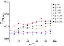
Fig. 20The variation law of the RMS pressure coefficient Cp,rms at a specific pressure tap as a function of azimuthal angle β

a) A1

b) A7

c) A9

d) A11

e) A15

f) A18

g) A22

h) A24

i) A26

j) A32

Pressure taps A9, A11, A15, A18, A22 and A24 are classified as category II. When $\alpha =$ 90°, curves are floated around 0.1, and when $\beta =$ 150°, the RMS pressure coefficient $C_{p,rms}$ is expected to undergo significant amplification under these conditions, and curves will be appeared sharp points. When $\alpha$ is the other angles, Curves are increased at first and then decreased with the increase of $\beta$ in the range of $\beta =$ 0°-90°. Curves are also increased at first and then decreased or tended to be flat with the increase of $\beta$ in the range of $\beta =$ 90°-180°. The maximum value of curves are reached at $\beta =$30° and minimum value of curves are reached at $\beta =$ 60° or $\beta =$75°.

Pressure taps A7 and A32 fall into Category III, where their RMS pressure coefficient $C_{p,rms}$ trajectories exhibit a distinct inflection point, first decreasing and then increasing with azimuth angle $\beta$, forming a concave-downward evolution pattern. Maximum value of pressure tap A7 is reached at $\beta =$ 180°, and maximum value of pressure tap 32 is reached at $\beta =$ 0°.

For $\alpha =$ 0°, the RMS pressure coefficient $C_{p,rms}$ trajectories of taps A1, A7, A26, and A32 oscillate between 0.1 and 0.6. Taps A1 and A7 exhibit marginally increasing trends, whereas A26 and A32 show slightly decreasing patterns. The remaining taps demonstrate stable $C_{p,rms}$ fluctuations within 0.1-0.2. The fluctuating wind pressure coefficient is increased significantly, and curves are shown an upward sharp point when $\beta =$150°.

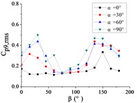
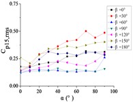
For $\alpha =$ 30°, the RMS pressure coefficient $C_{p,rms}$ trajectories of taps A1 and A26 oscillate between 0.3 and 0.6 as $\beta$ varies from 0° to 180°. These taps exhibit marked elevation in $C_{p,rms}$ relative to others within the 60° $\le \beta \le$ 20° sector due to boundary layer separation at the mirror's leading edge. The remaining eight taps demonstrate concave-upward trends ($C_{p,rms}$ first decreases then increases).

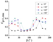
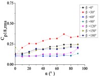
For $\alpha =$ 60°, The variation law of the RMS pressure coefficient $C_{p,rms}$ under these conditions is analogous to that observed at $\alpha =$30°, but the curve fluctuation of pressure taps A1 and A26 is not obvious than the curve fluctuation of other pressure taps, and the curve variation law of pressure taps A1 and A26 are tended to be horizontal.

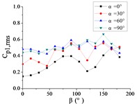
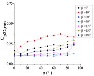
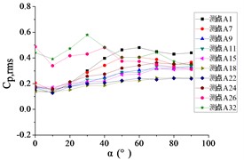
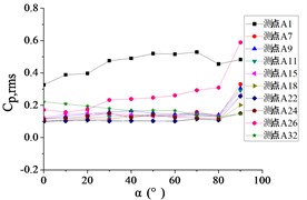
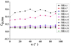
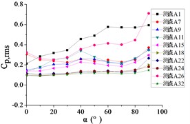
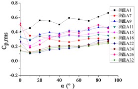
Fig. 21The variation law of root-mean-square (RMS) fluctuating wind pressure coefficients Cp,rms at ten positioned pressure taps as functions of azimuth angle β

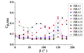
a) Elevation angle 0°

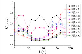
b) Elevation angle 30°

c) Elevation angle 60°

d) Elevation angle 90°

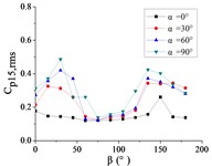
For $\alpha =$ 90°, the RMS pressure coefficient $C_{p,rms}$ at taps A1 and A26 exhibits marked elevation relative to other taps within the 60° $\le \beta \le$ 120° sector. Across the full $\beta \in$[0°, 180°] range, the remaining taps demonstrate concave-upward trends ($C_{p,rms}$ first decreases then increases) due to transient boundary layer separation at intermediate $\beta$ angles.

In summary, Taps A1 and A26 exhibit marked elevation in RMS pressure coefficient $C_{p,rms}$ relative to other sensors, and the variation law of A1 is not similar to that of A26. Conversely, the remaining taps demonstrate homogeneous $C_{p,rms}$ the variation law of curves is similar with each other.

4.3.2. Variation law of fluctuating wind pressure with elevation angle

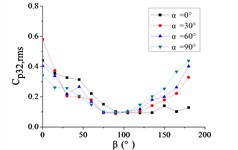
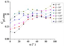
As shown in Fig. 22, the ten pressure taps are classified into three distinct categories. Category I includes taps A1 and A26, located at the windward and leeward edges of the mirror panel, with the increase of $\alpha$, curves are shown an increasing trend, and curves are basically reached the maximum value at $\alpha =$ 90° except for curves when $\beta =$ 0° and $\beta =$ 30°. When $\beta =$ 0° and $\beta =$ 30°, the RMS pressure coefficient trajectory of tap A1 exhibits an initial increasing trend with increasing elevation angle $\alpha$, and the maximum value is reached at $\alpha =$ 60°, and then is tended to be gentle. The RMS pressure coefficient trajectory of tap A26 demonstrates a concave-downward temporal evolution pattern as elevation angle $\alpha$ increases, the maximum value is reached at $\alpha =$ 20°.

Category II includes taps A7 and A32, with the increase of $\alpha$, curves are presented a horizontal distribution, curves are basically floated between 0.1 and 0.25 except for curves when $\beta =$ 0° and $\beta =$ 180°, and curves at $\beta =$ 0° and $\beta =$ 180° is significantly higher than the rest of curves. Curve of pressure tap A7 at $\beta =$ 180° and the curve of pressure tap A32 at $\beta =$ 0° are both floated around 0.5.

Category III includes taps A9, A11, A15, A18, A22 and A24. With the increase of $\alpha$, seven curves are divided into two categories, when $\beta =$ 0°, $\beta =$ 30°, $\beta =$ 150° and $\beta =$180°, these four curves are shown a gradual increase trend with the increase of $\alpha$, other three curves are horizontally distributed and floated around the fluctuating wind pressure coefficient of 0.1. Category III can be considered as a transitional stage between category I and category II. Different curves of pressure taps in category III have similar variation law as those in category I and category II respectively.

Fig. 22The variation law of the root-mean-square (RMS) fluctuating wind pressure coefficient Cp,rms at a specific pressure tap as a function of elevation angle α

a) A1

b) A7

c) A9

d) A11

e) A15

f) A18

g) A22

h) A24

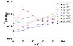
i) A26

j) A32

For $\beta =$ 0°, Taps A26 and A32 exhibit concave-downward $C_{p,rms}$ trajectories as $\alpha$ increases. Taps A18 and A22 maintain stable horizontal distributions ($C_{p,rms}\approx$0.15) across all $\alpha$, while the remaining taps demonstrate convex-upward trends ($C_{p,rms}$ first increases then plateaus).

For $\beta =$ 30°, Taps A26 and A32 exhibit concave-downward $C_{p,rms}$ trajectories as $\alpha$ increases. Taps A7 and A32 maintain stable horizontal distributions ($C_{p,rms}\approx$0.2) across all $\alpha$, while the remaining taps demonstrate convex-upward trends ($C_{p,rms}$ first increases then plateaus).

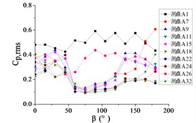
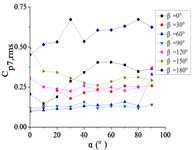
For $\beta =$ 60°, Taps A1 and A26 exhibit significantly elevated RMS pressure coefficients $C_{p,rms}$ relative to other sensors, demonstrating monotonically increasing trends with elevation angle α. Conversely, tap A32 shows a decreasing pattern, while other taps maintain stable fluctuations ($C_{p,rms}\approx$0.1). A sudden pressure surge occurs at $\alpha =$90°, creating an inflection point in the $C_{p,rms}$ trajectories at $\alpha =$80°.

For $\beta =$ 90°, Taps A1 and A26 exhibit significantly elevated RMS pressure coefficients $C_{p,rms}$ relative to other sensors, maintaining horizontal distributions at $C_{p,rms}\approx$0.5 and 0.35, respectively. The remaining taps demonstrate stable low-pressure plateaus ($C_{p,rms}\approx$0.1) across all elevation angles.

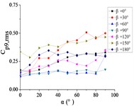
For $\beta =$ 120°, Taps A1 and A26 demonstrate monotonically increasing RMS pressure coefficients $C_{p,rms}$ with elevation angle $\alpha$, the peak values is higher than other sensors peak. Taps A7, A9, A11, and A15 maintain stable horizontal distributions ($C_{p,rms}\approx$ 0.2), while the remaining taps exhibit uniform low-pressure plateaus ($C_{p,rms}\approx$ 0.1).

For $\beta =$ 150°, Tap A7 exhibits a monotonically decreasing RMS pressure coefficient $C_{p,rms}$ with increasing elevation angle $\alpha$, while the remaining nine taps demonstrate moderate increasing trends. Among these, tap A1 maintains significantly elevated $C_{p,rms}$ (is much higher than other taps).

For $\beta =$ 180°, tap A1 maintains a stable horizontal RMS pressure coefficient $C_{p,rms}\approx$ 0.4 across all elevation angles $\alpha$. Conversely, other taps demonstrate monotonically increasing $C_{p,rms}$ trends, with tap A7 achieving significantly elevated values (is much higher than other taps).

Fig. 23The variation law of root-mean-square (RMS) fluctuating wind pressure coefficients Cp,rms at ten positioned pressure taps as functions of elevation angle α

a) Azimuth angle 0°

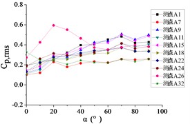
b) Azimuth angle 30°

c) Azimuth angle 60°

d) Azimuth angle 90°

e) Azimuth angle 120°

f) Azimuth angle 150°

g) Azimuth angle 180°

5. Conclusions

Based on wind tunnel test data, this study investigates the fluctuating wind force $F_{fluc}$ and fluctuating wind pressure coefficient $C_{p,fluc}$ of heliostat arrays, which are based on wind tunnel test, and the following main conclusions are obtained.

1) The 3D diagram of $C_{My,fluc}$ is similar to that of $C_{Fx,fluc}$, and the variation law is consistent, Which is because $F_x$ and $M_y$ is acted in the same direction, and $M_y$ is the result of the product of $F_x$ and the height of column. It is indicated that $C_{Fx,fluc}$ and $C_{My,fluc}$ are essentially the same. The 3D diagram of $C_{Mx,fluc}$ is also similar to that of $C_{Fy,fluc}$, and the variation law is consistent, which is also indicated that $C_{Fy,fluc}$ and $C_{Mx,fluc}$ are essentially the same.

2) The 3D diagram of the fluctuating wind force coefficient and the mean wind force coefficient can be compared, and the corresponding working conditions of the peak value of the fluctuating and average wind coefficient are also basically the same. Therefore, the study and analysis of heliostats need to be considered the peak value of fluctuating and average wind force coefficient and the corresponding working condition.

3) Within the $\beta =$ 0° sector with $\alpha \in$[0°, 90°] and $\beta =$30° sector with $\alpha \in$[60°, 90°], the temporal evolution patterns of heliostat arrays’ fluctuating wind pressure coefficients $C_{p,fluc}$ deviate significantly from isolated heliostat behavior due to wake-induced occlusion effects. Conversely, under other working conditions, the variation law of heliostats is similar to that of the isolated heliostat under other working conditions.

Through statistical analysis of 130 operational conditions, this study identifies the peak RMS fluctuating wind pressure coefficient $C_{p,rms,max}=$ 0.768 at tap A28 under the critical $\beta =$30°, $\alpha =$0° configuration. The corresponding contour map of $C_{p,rms}$ reveals coherent high-pressure regions at the mirror’s lower-left mid-edge. The position of the maximum of the mean wind pressure coefficient is consistent with that of the maximum of the fluctuating wind pressure coefficient. Therefore, the wind pressure resistance performance and related parameters of the mirror at this position should be analyzed and studied during the design of the heliostats.

Through analysis of heliostat fluctuating wind pressure coefficients $C_{p,rms}$, enabling classification of pressure taps into three categories. According to the variation law, pressure taps are divided into three categories, in which left-most pressure taps of the mirror surface are the category I, right-most pressure taps of the mirror surface is the category II, and other pressure taps of the mirror surface are the category III. The observed $C_{p,rms}$trends correlate strongly with tap positions and the position of the pressure tap is needed to be considered during research.