Analysis of vibration characteristics of automobile air conditioning piping system based on CFD

2.1. Control equations of fluid mechanics

The fluid motion within the air conditioning ducts of a car exhibits similarities to solid motion, governed by the principles of conservation of mass, momentum, and energy. The mathematical representation of these conservation laws forms the basis for establishing the control equations. The law of conservation of mass can be expressed as: over any given time interval, the mass of the fluid within the same infinitesimal control volume remains unchanged. In the context of air conditioning duct pipelines, the fluid is assumed to behave as a continuous and homogeneous medium, with its velocity and density being continuously differentiable functions in both space and time. Let the velocity at a certain point $\left(x,y\right)$ be $\left(u,v\right)$ and the temperature be $t$. The unsteady mass continuity equation and momentum equation can be respectively expressed as:

According to the law of conservation of energy, the unsteady energy equation in the two-dimensional space of air can be derived:

2.2. Turbulence model

The standard $k$-$\epsilon$ model was proposed by Launder and Spalding [8]. It determines the turbulent length and time scales by solving the transport equations of turbulent kinetic energy $k$ and its dissipation rate $\epsilon$. It has the advantages of strong robustness and fast convergence speed. However, the accuracy of this model is relatively poor and it is difficult to meet the accuracy requirements for non-standard turbulent problems. The RNG $k$-$\epsilon$ model takes into account the viscous effects between molecules at low Reynolds numbers and is generally used to predict moderately complex turbulent flows. Although the RNG $k$-$\epsilon$ model requires more computational time compared to the standard $k$-$\epsilon$ model, it offers higher accuracy and reliability. Therefore, it can be employed for the calculation of the steady-state flow field inside the air ducts of automotive air conditioning systems. The LES model distinguishes the velocity fields of large eddies and small eddies based on the self-similarity theory. By setting the grid size, small vortices are filtered out, and only large-scale vortices are calculated.

3.1. Geometric models

To efficiently calculate the fluid dynamics characteristics, ANSYS Fluent 2020R2 was employed. Since the focus is on calculating the internal flow field of the air duct pipeline, only the inner wall surface of the pipeline needs to be considered. However, due to the irregular cross-sectional shape and complex inner wall structure, the number of grids and the complexity of grid arrangement increase, leading to higher computational loads and costs.

To establish the fluid domain mesh model of the automotive air conditioning duct pipe, the surface meshing is carried out first. The surface mesh mainly consists of two types: triangular mesh and quadrilateral mesh. Due to the complex structure of the air conditioning duct pipe studied in this paper and the large curvature changes in some local areas, triangular mesh is used for surface meshing of the fluid domain of the air conditioning duct pipe. The surface mesh size is set to 3 millimeters according to the actual situation, and mesh refinement is carried out at the turning parts and areas with large curvature changes. After checking and optimizing the quality of the surface mesh, the volume mesh of the fluid domain is generated. The volume mesh is divided into structured mesh and unstructured mesh. Structured mesh has the advantages of good quality, simple structure, and fast convergence speed, but most structured meshes can only be applied to simple and regular-shaped models. Unstructured mesh has a slower generation speed, lower calculation accuracy and efficiency, but it can better adapt to complex geometric models. Since the size, shape and position of the mesh nodes in unstructured mesh are easier to control, compared with structured mesh, unstructured mesh has more mesh elements and higher requirements for computer hardware. Considering the advantages and disadvantages of the two types of meshes and the actual situation of the air conditioning duct pipe, the type of volume mesh selected in this paper is unstructured tetrahedral mesh. The mesh model of the air conditioning duct pipe is shown in Fig. 1(a). At the same time, to ensure calculation accuracy and accurately simulate the turbulent motion in the near-wall region, a boundary layer mesh is established. According to engineering experience, the number of boundary layer mesh layers is set to 7, and the size of the outermost layer is 0.2 millimeters, as shown in Fig. 1(b). The final number of mesh elements is approximately 792,508.

Fig. 1The result of meshing

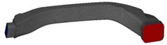
a) The grid model of the pipeline

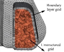
b) Boundary layer grid

3.2. Physical model and boundary conditions

After establishing the finite element model for the fluid calculation of the air conditioning duct, the boundary conditions and physical model of the model are set. In the computational fluid dynamics software, the inlet end of the air conditioning duct is set as a mass flow inlet, with the fluid flow direction along the normal direction of the inlet surface, uniformly flowing into the air conditioning duct. The outlet of the air conditioning duct is connected to the atmosphere, and the outlet is set as a pressure outlet, with the reference pressure being the standard atmospheric pressure and the relative pressure set to 0 Pa. The wall surface of the duct is set as an impermeable, adiabatic and no-slip wall.

Before conducting numerical simulation of the flow field, under the premise of ensuring the accuracy and authenticity of the calculation results, to facilitate the calculation and reduce the computational load, the following assumptions are made for the fluid domain:

(1) As the air flow velocity in the air conditioning duct is much lower than the local speed of sound, its compressibility can be ignored. It is assumed that the fluid in the air conditioning duct is an incompressible gas with a density of 1.225 kilograms per cubic meter, and the heat exchange process with the outside is ignored.

(2) It is assumed that the fluid flow is three-dimensional steady-state turbulence, and the slight deformation of the pipe wall caused by the fluid motion is ignored.

(3) It is assumed that the fluid is uniformly distributed at the inlet and outlet of the air conditioning duct.

Because of the relatively low air flow velocity, the flow can be categorized as incompressible or weakly compressible. In this case, the pressure-based solver is a more appropriate choice. The pressure-based solver utilizes a segregated solution algorithm that effectively addresses the coupling between pressure and velocity, demonstrating excellent stability and accuracy when solving low-speed flow problems. For air conditioning duct flows, the SIMPLEC algorithm is particularly suitable. It enhances the pressure correction equation based on the SIMPLE algorithm, improving convergence rates while maintaining high precision. This makes it especially effective for low Mach number flows, enabling rapid and accurate resolution of the coupling relationship between pressure and velocity.

4.1. Wall pressure distribution

In the computational fluid dynamics software, steady-state flow field simulation was conducted on the air conditioning duct pipe. After the simulation was completed, the average flow velocity and average pressure at the pipe inlet and outlet were calculated. The pressure loss of the pipe was the difference between the average pressure at the inlet and the average pressure at the outlet. As the average flow velocity of the fluid in the automotive air conditioning duct increases, the ratio of pressure loss is higher than the square ratio of the fluid flow velocity. Therefore, it is speculated that in addition to the friction loss along the duct, there are other sources of pressure loss within the duct. It is necessary to analyze the simulation results of the flow field in the air conditioning duct to explore the relationship between pressure loss and the flow field. After the steady-state flow field calculation of the automotive air conditioning duct converges, post-processing of the simulation results is carried out to obtain the static pressure distribution cloud diagrams of the automotive air conditioning duct under different working conditions, as shown in Fig. 2. It is observed that as the inlet flow rate increases, the static pressure on the pipe wall also rises. Pressure pulsations predominantly occur in two regions: first, at the front end of the pipe inlet, where the abrupt change in cross-sectional area induces turbulent airflow, creating a negative pressure zone within the pipe and thereby generating pressure pulsations. The energy loss at these pulsation points is relatively high, which tends to produce aerodynamic noise; second, at the bends of the pipe, where pressure variations are significant and unevenly distributed. Specifically, the pressure on the inner side of the pipe corner is lower, while it is higher on the outer side due to the centrifugal force acting on the gas flow during the turning process. During the flow process, frictional resistance along the pipe leads to energy dissipation, resulting in an uneven pressure distribution with distinct high-pressure and low-pressure zones. Consequently, it can be concluded that the pressure loss in the air duct increases with the rise in inlet flow rate, primarily attributed to the friction between the air and the pipe wall, as well as the negative pressure zones caused by air turbulence.

Fig. 2Simulation results of static pressure distribution

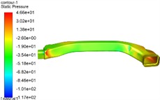
a) Inlet flow of 0.034 kg/s

b) Inlet flow of 0.050 kg/s

4.2. Air turbulence distribution

The steady flow field of the air conditioning duct pipe in the car was simulated. The streamline diagram and the velocity streamline diagram are shown in Fig. 3. The streamline diagram indicates the movement trajectory of the fluid, while the magnitude of the values in the velocity streamline diagram represents the movement speed of the fluid in different movement trajectories. It can be seen that the flow trend of the fluid is roughly the same under each working condition. In the area of sudden change in cross-sectional area near the entrance of the air conditioning duct, the fluid flow is rather disordered. Due to the significant change in the cross-sectional area of the pipe, the airflow may separate from the wall at this time, forming high and low pressure zones. Meanwhile, the airflow velocity changes significantly, causing turbulence and ultimately leading to the formation of a negative pressure zone. There are also obvious vortices at the outlet of the pipe. This is because when the gas flows through the corner of the pipe, the airflow accelerates. In the area behind the corner, the airflow separates from the wall, causing the gas to become disordered and form a vortex at the outlet.

Fig. 3Simulation results of streamline diagram of flow velocity

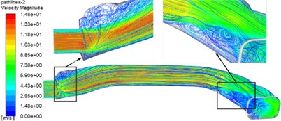
a) Inlet flow of 0.034 kg/s

b) Inlet flow of 0.050 kg/s

4.3. The distribution of aerodynamic sound sources

The noise calculated in the physical model of this paper mainly stems from the interaction between the gas and the pipe wall, thereby forming aerodynamic noise. Therefore, in the steady-state simulation, the distribution of dipole sound sources is mainly considered. For the distribution of surface sound sources of the automotive air conditioning duct under different working conditions, the broadband noise source model method (BNS) is adopted for calculation to predict the location of the aerodynamic sound source inside the automotive air conditioning duct. Simulation results of distribution of flow noise sources are shown in Fig. 4. It can be seen from the figure that under different working conditions, with the increase of airflow, the maximum value of noise sound pressure level significantly increases. The distribution area of noise sources hardly changes, and the noise is mainly concentrated in the area where the inlet cross-sectional area suddenly changes. As mentioned earlier, the pressure gradient and velocity gradient in this area are relatively large. The separation of air from the wall causes the fluid flow to become turbulent, generating aerodynamic noise in the process. The peak sound power level of the noise source increases with the increase of the inlet flow rate.

Fig. 4Simulation results of distribution of flow noise sources

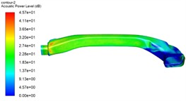
a) Inlet flow of 0.034 kg/s

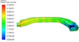
b) Inlet flow of 0.050 kg/s

4.4. The spectral characteristics of the noise at the air outlet

A monitoring point is set at 500 millimeters from the center of the outlet of the automotive air conditioning duct. The pressure pulsation information of the unsteady flow field obtained by computational fluid dynamics is combined with the FW-H acoustic analogy method to calculate the aerodynamic noise at the outlet of the duct. The noise sound pressure at the outlet of the car air conditioning duct obtained through calculation was converted into the reference sound pressure in the air to obtain the noise sound pressure level spectrum at the monitoring point, as shown in Fig. 5(a). Subsequently, in the finite element software, the noise sound pressure level at the outlet of the car air conditioning duct was converted into a sound pressure level that is more in line with the subjective response of the human ear, and its spectrum is shown in Fig. 5(b). The peak value of the noise sound pressure level at the outlet of the duct is about 54 dB, and the corresponding peak frequency is 100 Hz. The sound pressure level gradually decreases with the increase of frequency, and the spectral characteristics of the sound pressure level are consistent with the characteristics of a dipole sound source.

Fig. 5The spectral characteristics of the noise at the air outlet

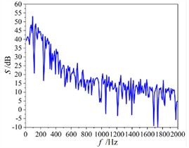
a) The noise sound pressure level spectrum

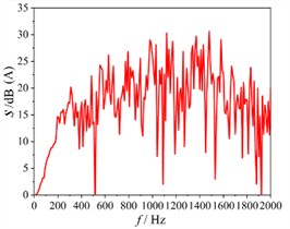
b) A-weighted sound pressure level spectrum

4.5. Transmission loss verification

To verify the reliability of the finite element model, the sound transmission loss test results based on the experimental scheme are shown in Fig. 6. It can be seen that the simulated and experimental values of the sound transmission loss of the air conditioning duct structure have an overall consistent trend and a good fit. The sound transmission loss is relatively low below 800 Hz, with the first two peaks approximately at 4.2 dB and 11.2 dB, corresponding to frequencies of approximately 240 Hz and 750 Hz, respectively. In the frequency band above 800 Hz, the sound transmission loss gradually increases with the increase in frequency, reaching a maximum of approximately 70 dB. Due to the limitations of the test bench, no vibration isolation treatment was carried out. When testing the sound transmission loss of the sound-absorbing structure, the slight vibration of the acoustic impedance tube caused fluctuations in the test results in the high-frequency range.

Fig. 6Transmission loss verification

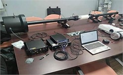
a) Experimental plan

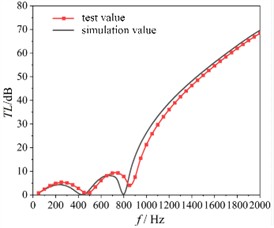
b) The result of transmission loss

References

-
K. V. V. Hoang, T. H. Quoc, and M. H. N. Thi, “Utilizing computational fluid dynamics (CFD) for simulating airflow and heat distribution to enhance thermal comfort in enclosed space,” Journal of Physics: Conference Series, Vol. 2949, No. 1, p. 012049, Feb. 2025, https://doi.org/10.1088/1742-6596/2949/1/012049
P. Zelenský, V. Zmrhal, M. Barták, and M. Kučera, “Simulation-aided development of a compact local ventilation unit with the use of CFD analysis,” Building Simulation, Vol. 17, No. 12, pp. 2233–2247, Oct. 2024, https://doi.org/10.1007/s12273-024-1183-9
Q. Ning, G. He, B. Li, and T. Li, “Theoretical and simulation analysis for R290 leakage from split-type air conditioners,” International Journal of Refrigeration, Vol. 166, No. 1, pp. 139–148, Oct. 2024, https://doi.org/10.1016/j.ijrefrig.2024.06.025
S. Dogra, P. Gulia, and A. Gupta, “Noise isolation in building HVAC system using recyclable plastic bottles,” Proceedings of the Institution of Mechanical Engineers, Part C: Journal of Mechanical Engineering Science, Vol. 238, No. 8, pp. 3327–3337, Oct. 2023, https://doi.org/10.1177/09544062231197391
L. Mao, H. Ma, D. Long, L. Zhang, and Q. Chen, “Low-frequency discontinuous noise diagnosis and reduction of air conditioner outdoor unit,” in Journal of Physics: Conference Series, Vol. 2660, No. 1, p. 012044, Dec. 2023, https://doi.org/10.1088/1742-6596/2660/1/012044
W. Cebulska, “Noise emissions in electric drive vehicles on the example of the Dacia spring electric car,” International Journal of Vehicle Noise and Vibration, Vol. 20, No. 3, pp. 242–255, Jan. 2025, https://doi.org/10.1504/ijvnv.2025.144735
M. Shaikh and A. Yadao, “Numerical and experimental investigation of vibration of a car chassis and its effect with road gradient on noise and response optimization with factorial design method,” Noise and Vibration Worldwide, Vol. 56, No. 1-2, pp. 38–51, Jan. 2025, https://doi.org/10.1177/09574565241306319
S. Parameswaran, S. Jayantha, and C. V. Chock, “A performance comparison of the standard k-ϵ model and a differential Reynolds stress model for a backward-facing step,” Numerical Heat Transfer, Part B: Fundamentals, Vol. 33, No. 3, pp. 323–337, Apr. 1998, https://doi.org/10.1080/10407799808915036
About this article
The authors have not disclosed any funding.
The datasets generated during and/or analyzed during the current study are available from the corresponding author on reasonable request.
The authors declare that they have no conflict of interest.