Numerical and experimental investigation of aerodynamic noise from automotive cooling fan module

2.1. Theoretical method

The key technique of large-eddy simulation is the separation between large and small scales. The governing equations for LES are obtained by filtering the time-dependent Navier-Stokes equations in the physical space. The filtering process effectively filters out eddies whose scales are smaller than the filter width or grid spacing used in the computations. The resulting equations thus govern the dynamics of the large eddies [4].

A filtered variable is denoted in the following by an overbar and is defined by:

where $\mathit{x}$ is one fluid particle coordinate in the fluid domain, $\mathit{x}\text{'}$ is another fluid particle coordinate in the fluid domain, $D$ is the fluid domain, and $G$ is the filter function that determines the scale of the resolved eddies:

where $V$ is the control volume. The filter function $G(\mathit{x}-\mathit{x}\mathrm{\text{'}})$ implied here is then:

Filtering the Navier-Stokes equations leads to additional unknown quantities. In the following the theory will be outlined for the incompressible equations. The filtered incompressible momentum equation can be written in the following way:

where $i$ and $j$ are two orthogonal directions. ${\tau }_{ij}$ denotes the subgrid-scale stress. It includes the effect of the small scales and is defined by:

The large scale turbulent flow is solved directly and the influence of the small scales is taken into account by appropriate subgrid-scale (SGS) models. An eddy viscosity approach is used that relates the subgrid-scale stresses ${\tau }_{ij}$ to the large-scale strain rate tensor ${\stackrel{-}{S}}_{ij}$ in the following way:

where the eddy viscosity $v_{sgs}$ represents all turbulent scales, the subgrid-scale viscosity only represents the small scales. In this study, the sub-grid scale velocity fluctuations are modeled with a dynamic Smagorinsky model. The schematic geometrical model for Eqs. (1)-(6) can be referred in [16].

2.2. Aerodynamic modeling

The reasonable aerodynamic model is the important foundation of numerical aeroacoustic prediction. The investigated model is a single 7-blade automotive cooling fan module which is presented in Fig. 1(a). The fan flow field is mainly affected by the blade and the shroud frame, therefore some details are simplified and the simplified fan module is shown in Fig. 1(b).

Fig. 1Cooling fan module model

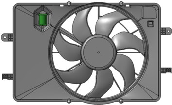
a) Original model

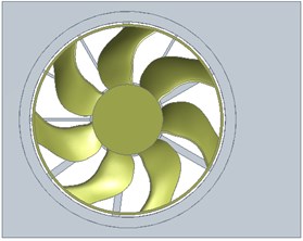
b) Simplified model

The aerodynamic model is shown in Fig. 2(a). Rotating domain and stationary domain are established in the CFX 15.0. According to the noise experiment environment, the total length of the external stationary domain 2000 mm. Inlet and outlet are on the front and back sides of the external stationary domain.

Fig. 2Aerodynamic model

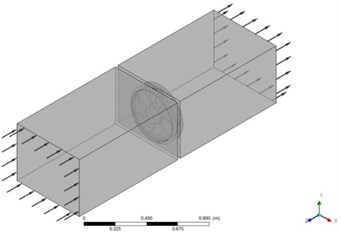
a) Computational domain

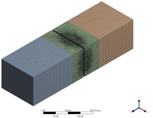
b) FEM model

The FEM model is shown in Fig. 2(b), which is generated in ICEM CFD 15.0. Considering the complexity of the blade surface, hexahedral inflation layer grids with fine resolution are created near the surface of blades for the accuracy of capturing the pressure fluctuations. Pyramid and tetrahedral grids are used in the rest area of rotational domain. And in the middle part of stationary domain, tetrahedral grids are generated for improving the computational efficiency. Hexahedral grids are created in the front and rear parts of stationary domain, whose geometry are relatively simple, to increase both computational accuracy and efficiency. The number of elements and nodes are given in the Table 1.

The flow field is composed of rotational domain and stationary domain, so the interface between two domains should be considered. The interfaces of two domains are set as “Frozen Rotor” in steady computation and “Transient Rotor Stator” or called as “Sliding mesh method” is set in unsteady computation to capture the transient relative motions between rotors and stators. In this approach, the interface position is updated each physical time step and the flow variables on the interfaces are transferred to each other through the meshes of the interfaces.

The inlet boundary condition is defined as “static pressure condition” as 0 Pa to represent the ambient pressure and the outlet boundary condition is defined as “static pressure condition” as 0 Pa as well. The wall condition is defined as “adiabatic, no slip condition”. Because the flow Mach number is below 0.2, the gas is defined as non-compressible gas. 3 cases are set to capture the aerodynamic noise source information in 3 different operating conditions. The case setting is shown in Table 2.

The unsteady computation is based on the steady state flow field result. The cut-off frequency is set as 2500 Hz, so according to Nyquist sampling theorem the sampling interval is set as 0.0002 s. The maximum number of timesteps is set as 10,000. In order to ensure the convergence of flow field computation, the monitors of coefficient loop convergences are set up, including pressure and velocity at the both inlet and outlet.

2.3. Results and discussion

Fig. 3 and Fig. 4 show the fluctuating pressure field on the pressure and the suction side of fan and shroud in Case 3. The pressure of suction side is negative but the pressure near the blade leading edge is positive. The turbulent flow on the pressure side presents more significant fluctuations than those observed on the suction side. In addition, there are more significant interaction in the areas close to the trailing edge than the leading edge of the blades. The aerodynamic noise is mainly generated by the interaction between the flow and the leading edges. The pressure field on the shroud surface is very inhomogeneous, which demonstrates the shroud affects the air distribution behind the fan blade surface significantly. The interaction between the fan and the shroud leads to pressure fluctuation and vortex disturbance, which are the major aerodynamic noise sources areas.

Fig. 5 and Fig. 6 depict the turbulence kinetic energy and turbulence eddy frequency distributions on the cross-sectional plane near the fan blades and the stability bars in Case 3. It is acknowledged that the turbulent kinetic energy and turbulence eddy frequency are representations of the magnitude of broadband noise sources [8]. Interestingly, the turbulence kinetic energy and turbulence eddy frequency distributions have similar patterns, which reach the maximum near the tailing edges and the inside of the ring. These intense contours may be a result of the fierce interaction of the air in the blade passage with the flow through shroud. According to the vortex sound theory, these eddies make great contributions to the aerodynamic noise generation.

Fig. 3Pressure field on fan surface

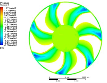
a) Suction side

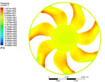
b) Pressure side

Fig. 4Pressure field on shroud surface

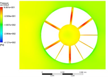
a) Suction side

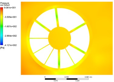
b) Pressure side

Fig. 5Turbulence kinetic energy

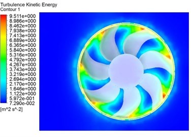
a) Near the fan blades

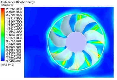
b) Near the stability bars

3.1. Theoretical method

The aeroacoustic analogy allows to find an expression for the incident acoustic field generated by a rotating fan at the blade passing frequency and harmonics. Some assumptions are taken into account to develop Lowson formula [17]: the fluid is incompressible, the flow is subsonic with a low Mach and high Reynolds numbers and the point $O$ defining the observer is located in a distance supposed very large in front of that defining the source $S$, which is shown in Fig. 7. When stator is at the outlet, axial and tangential contributions of the radiated pressure at frequency $mB\mathrm{\Omega }$:

Fig. 6Turbulence eddy frequency

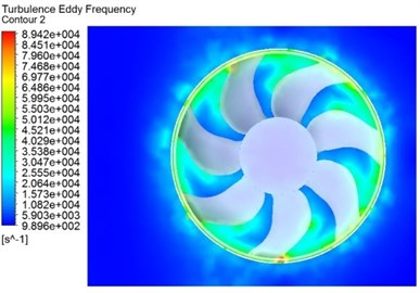
a) Near the fan blades

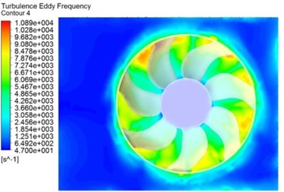
b) Near the stability bars

Radial contribution:

where $m$ is the harmonic number, $B$ is the number of rotor blades, $\mathrm{\Omega }$ is the rotation speed, $R$ is the distance from the observer, $c_0$ is the speed of sound, $F_{mB}$ is the Fourier series of the total force on a compact blade segment, $M$ is the rotational Mach number, $\theta$, $\phi$ and $\gamma$ are defined in Fig. 7, $V$ is the number of stator vanes. ${\alpha }_0$ is the phase angle.

The pressure field is captured from the loading force on a reference rotor blade or a reference stator vane. The force can be computed from the pressure fluctuations in time domain obtained from previous CFD unsteady computation. The resulting loading force is applied at one point of the blade. The representation of the fan by a single fan source is a good approximation when the size of the blades is small compared to the wavelength. When the size of the blade is very large and the fan cannot be considered as a compact source, the blade can be subdivided in a set of segments where each segment can be replaced by an equivalent source.

Fig. 7Reference of the fan

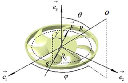
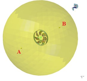
Fig. 8Acoustic model

3.2. Aeroacoustic modeling

The acoustic model is established in the commercial program LMS Virtual. Lab 13.1. Considering the impact of shroud to the noise propagation, acoustic boundary element mesh is established by Boundary Element Method, where the sound pressure is represented on the boundary elements. Fig. 8 depicts the boundary element mesh of the domain, where a cylinder field point mesh is created to represent the shroud and a spherical field point mesh ($R=$ 1 m) is established around the fan as the acoustic response field. In addition, two receiving points are set at inlet that 1 m before the fan center as point A and at outlet 1 m behind the fan center as point B along the rotation axis.

Fan blade surface pressure fluctuation data are imported and the acoustic fan source equivalence is created. Fan can be modelled as a cloud of rotating point dipoles in the acoustic model. With the new feature in LMS Virtual. Lab 13.1, automatic detection of blades and generation of segments (point dipoles) are accessible. In this study the maximum analysis frequency is set as 2500 Hz so that one blade is equivalent to 11 point rotating dipoles automatically. Because the size of the blades is small compared to the wavelength, it is reasonable in both simulation accuracy and efficiency. As a result the entire fan is represented by 77 point rotating dipoles as aeroacousitc sources.

3.3. Results and discussion

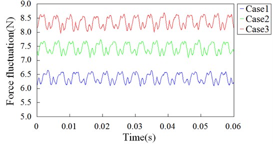
The blade forces are visualized for the verification of their consistency. The variations of the axial force fluctuation over the blades over 0.06 s in 3 cases are presented in Fig. 9. 13, 14 and 15 peaks corresponding to the 7 fan blades occur over 0.06 s in Case 1, Case 2 and Case 3. With the increase of rotation speed, the force fluctuation both in average amplitude and in terms of fluctuation is also increasing. In addition, the most significant force fluctuation appears in Case 3. It is so logical for an axial fan that the radial and tangential components of the forces are negligible compared to axial component.

Fig. 9Axial force fluctuation over fan blades vs. time in 3 cases

The two-dimensional sphere sound pressure distributions of Case 3 from 1×Blade Passing Frequency (BPF) to 3×BPF are shown in Fig. 10. The axial dipole characteristic at 1×BPF to 2×BPF are obvious and sound power is more concentrated. 3×BPF sound field still demonstrates dipole characteristic, but the axial deflection occurs.

Tonal noise and broadband noise are computed in the time domain and by the Fourier transform the SPL spectrums are predicted. Fig. 11 demonstrates the predicted SPL spectrums in 3 cases at two receiving points. As can be seen the SPL under 500 Hz is low while fluctuating around 30 dB after 500 Hz. There are obvious noise peaks at 1×BPF to 9×BPF, and at 2×BPF the maximum peak occurs. Tonal noise is higher than broadband noise, which shows tonal noise occupies the major part of the aerodynamic noise at high rotation speed. At the same receiving point, tonal noise and broadband noise increases with rotation speed.

Fig. 10Predicted sound pressure distribution at different BPF

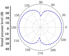
a) 1×BPF

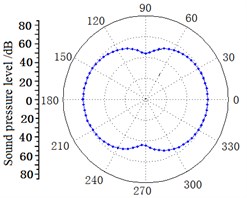
b) 2×BPF

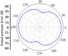
c) 3×BPF

Fig. 11Predicted SPL spectrums at two receiving points

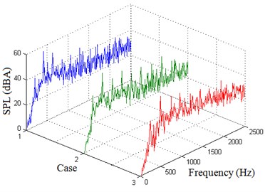
a) Point A

b) Point B

For the verification of the noise prediction of the cooling fan module, the noise experiment of the cooling fan module is carried out in the semi-anechoic chamber. The semi-anechoic chamber is 4.0 m×3.5 m×3.8 m and the environmental noise is below 20 dB (A). Noise experiment equipment is shown in Fig. 12. B&K 3560 multichannel analyzer and two microphones are used in the experiment. The microphone A and B are 1 m over the ground and the positions are as same as receiving point A and B in the simulation, which are demonstrated in Fig. 13.

Fig. 12Noise experiment equipment

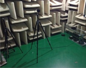
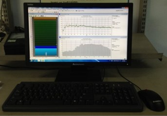
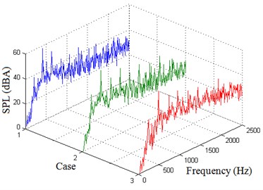
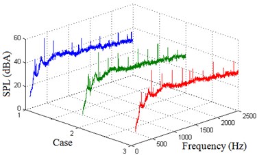
Fig. 14 demonstrates experimental SPL spectrum results in 3 cases at two receiving points. As can be seen in all cases, the SPL of tonal noise prediction and experimental results agree well. There are larger fluctuations in broadband noise prediction results than experimental results, but the trend remains in good agreement with the experimental values, which verifies the accuracy of the numerical prediction of aerodynamic noise.

Fig. 13Top view of the noise experiment environment

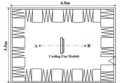
Fig. 14Experimental SPL spectrums at two receiving points

a) Point A

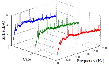
b) Point B

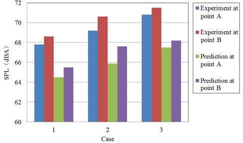
Fig. 15 is a comparison of the predicted results and the experimental results of the sound pressure level at two receiving points. Inlet and outlet sound pressure levels increase with increasing flow rate, and SPL in Case 3 is maximized. SPL at the export is larger than the import, which demonstrates that the impact of the dipole source to outlet is larger than inlet. SPL simulation results are smaller than the experimental results and the average relative error is less than 5 %. Part of these differences between the experimental and the predicted results can be attributed to the following reasons. On one hand, the fan blades are set as the only sources of the aerodynamic noise while the shroud frame noise, which is considered as stator noise, is neglected. On another, only aerodynamics noise is taken into account in the simulation. However, the experiment results contain aerodynamics noise and other noises, such as the vibration noise and electromagnetic noise from the electromotor of cooling fan module. Therefore in the next step of aeroacoustic simulation, both the stator noise and flow-introduced vibration noise should be taken into consideration to make the prediction results more accurate.

Fig. 15SPL comparisons between the experiment and prediction at two receiving points