Dynamic and static study of the fluid-structure interaction problem on elastic box plate

1. Introduction

This paper deals with the mathematical analysis of problems dealing with steady fluid-structure interactions (FSI) phenomena by a new theoretical method. Our attention is the both dynamic and static deformations, static velocity and pressure when flow around the elastic bodies immersed in a fluid stream. Such immersed-body flows are commonly encountered in engineering studies: aerodynamics (airplanes, rockets, projectiles), hydrodynamics (ships, submarines, torpedoes), transportation (automobiles, trucks, cycles), wind engineering (building, bridges, water towers, wind turbines), and ocean engineering (buoys, breakwaters, pilings, cables, moored instruments) [1-3]. And these phenomena have been studied by many authors over the past few years from different points of view (theoretical algorithm, numerical analysis and simulation, etc) [4-7].

Typically, fluid and structure are given in different coordinate systems making a common solution. Fluid flows are given in Eulerian coordinates whereas the structure is treated in a Lagrangian framework. We use united Lagrangian-Eulerian method to present the deformation, pressure and velocity of flow of a nonviscous, incompressible fluid around an elastic box plate. It is a new method of where fluid and structure equations are given in their preferred reference frames. The coupling between the fluid and structure domains is kinematic and dynamic conditions at the body surface. The effect of deformation of the elastic plate is taken into account by united Lagrangian-Eulerian method. It is different from the classic fluid mechanics.

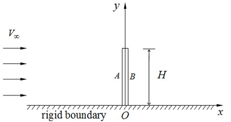
A schematic of steady and irrotational flow of a nonviscous, incompressible fluid around an elastic box plate is shown in Fig. 1. Thus the effect of viscosity, compression and fluid rotation are neglected. An orthogonal $xyz$ coordinate system is used, and all investigated values of the plate and fluid are assumed to be functions independent of the coordinate $z$. The surfaces $A$ and $B$ of box plate are elastic, and the others are rigid. The surface $A$ is very close to $B$. This article mainly studies the simply supported plate $A$. The pressure inside of the box plate is assumed to be constant. The physical parameters of the two-dimensional plate are: the mass density ${\rho }_s$, length $H$, thickness $h$ and bending stiffness $D=Eh{}_{\mathrm{}}{}^3/\left[12\right(1-{\nu }^2\left)\right]$, where $E$ is Young’s modulus and $\nu$ is the Poisson ratio.

Fig. 1Schematic of flow around an elastic box plate

2. Dynamic equations

In this section the governing equations for the separate fluid and structural problems are presented together with the surface coupling conditions.

2.3. United Lagrangian-Eulerian method

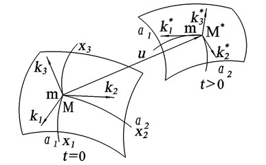
The structure and fluid state equations can be written in Lagrangian and Eulerian reference frames, respectively. The coupling between the fluid and structure are kinematic and dynamic conditions at the surface, as illustrated in Fig. 2. The kinematic condition is the no slip condition, i.e., continuity in velocity, and the dynamic condition is surface continuity in tractions [9]. They are written as:

5

$\mathbf{v}\cdot k_3^{*}=\left(\partial \mathbf{u}/\partial t\right){\mathbf{k}}_3^{*},\left(M^{*}\right),$

6

$Z=\left(p-p_i\right){\mathbf{k}}_3^{*},\left(M^{*}\right),$

in which $\mathbf{v}$ is the velocity vector of fluid flow, $\mathbf{u}$ is the displacement vector of structure, $p$ and $p_i$ are the pressures along outward and inward normal directions. ${\mathbf{k}}_3^{*}$ is the outward unit normal vector to the structure at the surface between structure and fluid in the deformed configuration. This can be expressed as:

7

${\mathbf{k}}_3^{*}=E_1{\mathbf{k}}_1+E_2{\mathbf{k}}_2+E_3{\mathbf{k}}_3,$

8

$E_1=e_{12}{\omega }_2-\left(1+e_{22}\right){\omega }_1,E_2=e_{21}{\omega }_1-\left(1+e_{11}\right){\omega }_2,$
$E_3=\left(1+e_{11}\right)\left(1+e_{22}\right)-e_{12}{e}_{21},$

9

$e_{11}=\frac{\partial u_1}{H_1\partial {\alpha }_1}+\frac{u_2}{H_1{H}_2}\frac{\partial H_1}{\partial {\alpha }_2}+k_{11}{u}_3,e_{12}=\frac{\partial u_2}{H_1\partial {\alpha }_1}-\frac{u_1}{H_1{H}_2}\frac{\partial H_1}{\partial {\alpha }_2}+k_{12}{u}_3,$

10

${\omega }_1=\frac{\partial u_3}{H_1\partial {\alpha }_1}-k_{11}{u}_1-k_{12}{u}_2.$

Fig. 2Two positions of structural elements in space

The scalar contact conditions are given by:

11

$\left(\frac{\partial u_1}{\partial t}-v_1\right)E_1+\left(\frac{\partial u_2}{\partial t}-v_2\right)E_2+\left(\frac{\partial u_3}{\partial t}-v_3\right)E_3=0,\left(M^{*}\right),$

12

$Z_1^{*}=Z_2^{*}=0,Z_3^{*}=p-p_i,\left(M^{*}\right),$

where $v_i^{}$ and $Z_i^{}$ ($i=$ 1, 2, 3) are the projections of the velocity and the external force vector at point $M^{*}$. The velocity function $\mathbf{v}\left(\mathbf{r}\right)$ and pressure function $p\left(\mathbf{r}\right)$ can be written in an Eulerian reference frame at point $M$. The function $\mathbf{v}(\mathbf{r}+\mathbf{u})$ and $p(\mathbf{r}+\mathbf{u})$ can be expressed in terms of Taylor expansion of $\mathbf{v}\left(\mathbf{r}\right)$ and $p\left(\mathbf{r}\right)$. Then the kinematic and dynamic conditions can be written as [9]:

13

$\left(\frac{\partial u_1}{\partial t}-V_1\right)E_1+\left(\frac{\partial u_2}{\partial t}-V_2\right)E_2+\left(\frac{\partial u_3}{\partial t}-V_3\right)E_3=0,\left(M\right),$

14

$Z_1^{*}=Z_2^{*}=0,Z_3^{*}=p+\frac{u_1}{h_1}\frac{\partial p}{\partial x_1}+\frac{u_2}{h_2}\frac{\partial p}{\partial x_2}+\frac{u_3}{h_3}\frac{\partial p}{\partial x_3}+\frac{u_1^2}{2h_1^2}\frac{\partial {}^{2}p}{\partial x_1^2}+\dots ,\left(M\right),$

where $V_1$, $V_2$ and $V_3$ are the projections of the velocity vector at point $M$. They can be expressed as:

15

$V_1=v_1+\frac{u_1}{h_1}\left[\frac{\partial v_1}{\partial x_1}+\frac{\partial h_1}{h_2\partial x_2}{v}_2+\frac{\partial h_1}{h_3\partial x_3}{v}_3\right]+\frac{u_2}{h_2}\left[\frac{\partial v_1}{\partial x_2}-\frac{\partial h_2}{h_1\partial x_1}{v}_2\right]$
$+\frac{u_3}{h_3}\left[\frac{\partial v_1}{\partial x_3}-\frac{\partial h_3}{h_1\partial x_1}{v}_3\right]+V_1^{\text{'}}\left(\frac{u_1^2}{h_1^2}\frac{\partial v_1}{\partial x_1},\cdots \right).$

The complex functions $V_1^{\text{'}}$, $V_2^{\text{'}}$, $V_3^{\text{'}}$ are the velocity components concerned with the quadratic expressions of Taylor expansions.

Taking into account the minor deformation of the structure, the kinematic condition of the structure can be expressed as:

16

$v_3=\frac{\partial u_3}{\partial t}+{\omega }_1{v}_1+{\omega }_2{v}_2-\frac{u_1}{h_1}\left[\frac{\partial v_3}{\partial x_1}-\frac{\partial h_1}{h_3\partial x_3}{v}_1\right]-\frac{u_2}{h_2}\left[\frac{\partial v_3}{\partial x_2}-\frac{\partial h_2}{h_3\partial x_3}{v}_2\right]$
$-\frac{u_3}{h_3}\left[\frac{\partial v_3}{\partial x_3}+\frac{\partial h_3}{h_1\partial x_1}{v}_1+\frac{\partial h_3}{h_2\partial x_2}{v}_2\right].$

The dynamic conditions can be expressed as:

17

$Z_1^{*}=Z_2^{*}=0,Z_3^{*}=p+\frac{u_1}{h_1}\frac{\partial p}{\partial x_1}+\frac{u_2}{h_2}\frac{\partial p}{\partial x_2}+\frac{u_3}{h_3}\frac{\partial p}{\partial x_3}.$

In this study, for the box plate, $u_3=w$, $u_2=u$, ${\alpha }_2=x_2=y$, ${\alpha }_3=x_3=x$, $h_2=\text{1}$, $h_3=\text{1}$, $H_2=\text{1}$, $H_3=\text{1}$, substituting these terms into Eqs. (16) and (17), the kinematic and dynamic conditions can be written as:

18

$\frac{\partial \phi }{\partial x}=\frac{\partial w}{\partial t}+\frac{\partial w}{\partial y}\frac{\partial \phi }{\partial y}-w\frac{{\partial }^2\phi }{\partial x^2}-u\frac{{\partial }^2\phi }{\partial x\partial y},$

19

$Z_1=p+w\frac{\partial p}{\partial x}+u\frac{\partial p}{\partial y}-p_i.$

Thus the dynamic equation of the plate is expressed as:

20

$D\frac{{\partial }^{4}w}{\partial y^4}+{\rho }_{s}h\frac{{\partial }^{2}w}{\partial t^2}=p+w\frac{\partial p}{\partial x}+u\frac{\partial p}{\partial y}-p_i,(x=0).$

This article studies minor deflection of plate, then displacement $u$ is neglected.

3. Theoretical solutions of dynamic equations

We study the dynamic and static fluid- structure interactions problems. When the plate is assumed to be absolutely rigid ($w_1\equiv 0$), the relative velocity potential ${\phi }_1$ and the pressure $p_1$ of fluid are introduced. The velocity potential ${\phi }_2$ and the pressure $p_2$ which concerning the thin plate bend, $w_2$ is the deflection of elastic plate, then we obtain:

Then substituting Eq. (21) into Eqs. (2)-(4) and (18)-(20), the following expressions for ${\phi }_1$ and $p_1$ can be written:

The following expressions for ${\phi }_2$ and $p_2$ can be written:

Eq. (20) can be written as:

The expression of velocity potential ${\phi }_1$ is given by [10]:

Substituting Eq. (31) into (23), the pressure $p_1$ can be written as:

Let us consider the general forms of the displacement and velocity potential:

where $W_n$ and $A_i$ are coefficients to be determined, $\mathrm{c}\mathrm{o}\mathrm{s}\theta =x/\sqrt{x^2+y^2}$, $\omega =2\pi f\text{,}$$f$ is frequency of disturbance force, $j$ is imaginary unit. Taking into account the minor deflection of the plate, one item is used for ${\phi }_2$.

Substituting Eqs. (33) and (34) into (29) and (30), and using Taylor expansions at $y=H/2$, the following expressions can be written:

The solutions of the set of Eqs. (35)-(37) are:

where:

The solutions of the corresponding static equations are:

4. Numerical examples and discussion

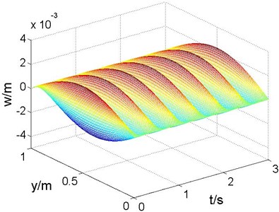
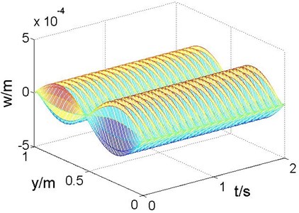
In this section, numerical examples are presented. The test elastic plate and fluid flow have the following characteristics: plate mass density ${\rho }_s=\mathrm{}$7850 kg/m³, thickness $h=\mathrm{}$1×10^-3 m, length $H=$1 m, Young’s modulus $E=$200×10⁹ N/m², Poisson’s ratio $\nu =\text{0.3,}$ flow velocity $V_{\infty }=\mathrm{}$0.06 m/s, mass density ${\rho }_{\infty }=\mathrm{}$1000 kg/m³, pressure $p_{\infty }=$1×10⁵ Pa. The obtained time histories of the deflection and the vibration velocity are shown in Fig. 3 and Fig. 4, respectively. These figures show that the modal shapes of the different frequencies of the vibration plate are different.

The corresponding statics results are shown in Fig. 5-Fig. 10.

Fig. 5 shows the deformation w by varying the length of plate. The deformation $w$ is the maximum value near the middle of the plate, closer to $y=\text{0}$. And $w$ is zero at $y=0$, $H$, respectively.

In Fig. 6, the pressures of the plate surface are given for different length of plate. To examine the effect of deformation, we compared the pressure considering the effect of deformation and without the effect (Fig. 7). It shows the pressures considering the effect of deformation are very close to those without the effect of deformation. Thus the effect of deformation can be ignored for the problem of minor deformation.

We define the pressure coefficient $C_p=2(p-p_{\infty })/{\rho }_{\infty }{V}_{\infty }^2$. Fig. 8 shows the positive pressure coefficient changes slightly from $y=\text{0}$. The pressure coefficient is negative near $y=H$ and the value changes sharply.

Fig. 3Time history of the deflection with f= 2 Hz and f= 10 Hz

a)$f=$ 2 Hz

b)$f=$ 10 Hz

Fig. 4Time histories of the vibration velocity

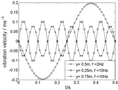
Fig. 5Deformations of plate for H= 0.9 m, 1.0 m and 1.1 m

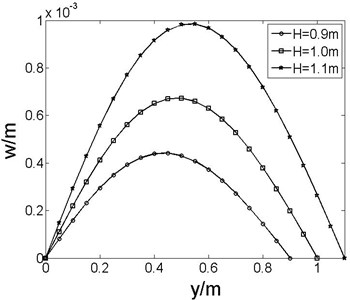
Fig. 6Pressure of the plate surface

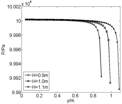
Fig. 7Comparison the pressure of plate surface considering the effect of deformation and without the effect

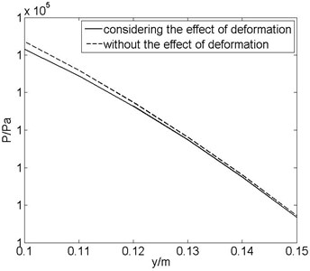
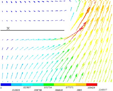
Fig. 9 and Fig. 10 illustrate the fluid velocity from united Lagrangian-Eulerian method. It is seen that a stagnation point where $V=\text{0}$ exists the point $y=\text{0}$ on the front side of the box plate. Bernoulli's equation predicts a maximum pressure at stagnation point because the velocity is zero at such points. A maximum velocity, and thus a minimum pressure, would exist near the plate tips.

An example of finite element method (FEM) is presented to illustrate the united Lagrangian-Eulerian method for FSI problems discussed in the present paper. The FEM model is depicted in Fig. 11. On the inflow boundary (the bottom) the velocities are prescribed $V_x=$0.06 m/s and $V_y=\text{0}$, the displacements are prescribed zero. On the outflow boundary (the top) the pressure is zero. The fluid displacement $U_y$ (for $y$ axes) and velocity $V_y$ of flow are zero on the left and the right boundaries. The domain has the dimensions 2 m×2 m. The model consists of 60802 nodes and 60000 elements: fluid 141 elements for the fluid and plane 42 elements for the structure. The time step is 0.1 s.

Fig. 8Pressure coefficient of plate surface for H= 0.9 m, 1.0 m and 1.1 m

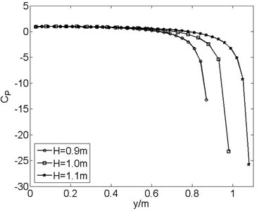
Fig. 9Fluid velocity with V∞= 0.06 m/s and H= 1 m

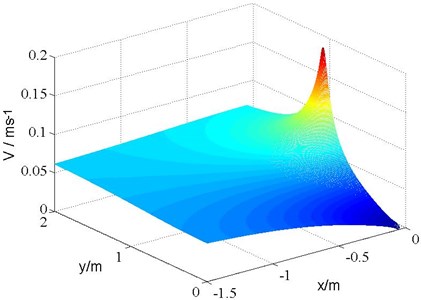
Fig. 10Vx-x, Vx-y, Vy-x and Vy-y curves when V∞= 0.06 m/s and H= 1 m at various values of x or y

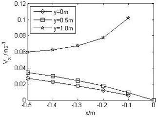
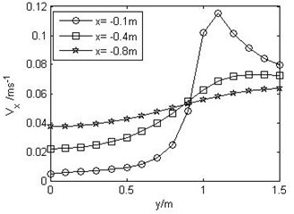
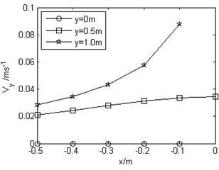
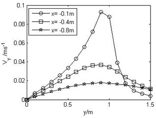
Fig. 12 and Fig. 13 present the deformation of the plate and the velocity vector of the fluid, which are obtained from FEM. It is seen that FEM solutions are consistent with theoretical results.

Fig. 11FEM model of fluid flow around an elastic plate

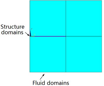
Fig. 12Deformation profile of FEM

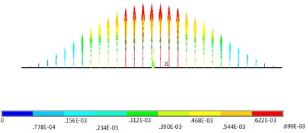
Fig. 13Velocity vector profile of FEM

5. Conclusions

Flow around an elastic box plate provides an example in this study. To united Lagrangian-Eulerian method, the plate and fluid state equations can be written in Lagrangian and Eulerian reference frames, respectively. The coupling between the fluid and plate domains is kinematic and dynamic conditions at the surface. The theoretical deformation, pressure and velocity of the problem of flow around an elastic box plate have been derived. Numerical results reveal the streamlines with very high velocities and low pressures near the plate tips. It is shown that the united Lagrangian-Eulerian method is an effectively method for the problem of elastic structure acted by ideal fluid flow.