Simulation data-driven intelligent fault diagnosis based on attention mechanism and transfer learning

Qiu, Xiaorong; Xu, Ye

doi:10.21595/jve.2025.25088

Journal of Vibroengineering

Browse Journal

Submit article

Published: February 20, 2026

Check for updates

Simulation data-driven intelligent fault diagnosis based on attention mechanism and transfer learning

Xiaorong Qiu¹

Ye Xu²

^{1, 2}School of Internet of Things Engineering, Wuxi Institute of Technology, Wuxi, 214121, China

Corresponding Author:

Xiaorong Qiu

Cite the article Download PDF

Article in Press

Downloads 200

Abstract

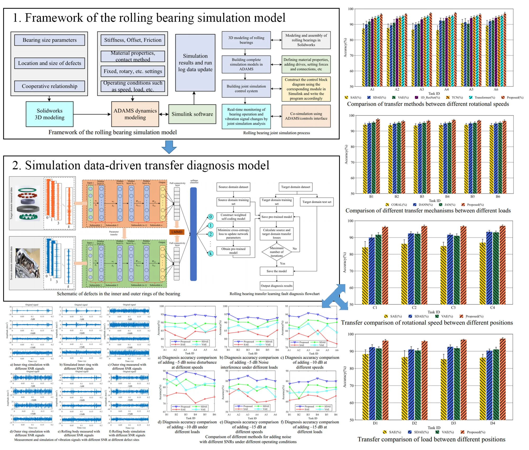
In this paper, a simulation data-driven intelligent fault diagnosis algorithm based on attention mechanism and transfer learning is proposed to address insufficient fault data, low diagnostic accuracy, and inefficiency in rolling bearing monitoring under cross-condition and cross-location scenarios. To overcome the lack of real fault data, a dynamic vibration-response model is constructed through analysis of bearing and fault dynamics, generating high-fidelity fault signals across multiple operating conditions. Based on this, a diagnostic model is developed using a self-attention–assisted weighted autoencoder, where the proposed weighted autoencoder integrates a self-attention mechanism and a weight allocation mechanism and the former captures inter-feature dependencies while the latter adaptively reweighting feature contributions to enhance fault-discriminative representations. Therefore, the diagnostic model can assign corresponding weights to different importance features according to the constructed self-attention mechanism-assisted weighted self-encoding feature extraction model, effectively avoiding the problems of insufficient diagnostic accuracy and low diagnostic efficiency caused by feature redundancy and difficulty in distinguishing the importance of rolling bearing faults. Furthermore, the local maximum mean discrepancy (LMMD) method is applied to align both global and sub-domain distributions between simulated and measured data. By synthesizing cross-condition and cross-location simulated signals with real measurements, an LMMD-based intelligent transfer diagnosis model is built to enhance generalization and robustness against large distribution discrepancies. Finally, the stability and robustness of the proposed method are validated by analyzing the transfer learning performance and anti-noise disturbance ability across different operating conditions and locations.

1. Introduction

As key component extensively used in rotating machinery such as gearboxes, fans, engines, and high-speed trains, rolling bearings play a crucial role in transmitting motion and maintaining safe and stable operation of equipment. They are often referred to as the “joints of industry” [1-7]. However, during actual operation, rolling bearings are subjected to complex and dynamic working environments, influenced by various external factors that induce high-intensity working frequencies, making them highly susceptible to failure. Studies indicate that over 30 % of faults in rotating machinery are attributed to bearing failures, with this figure rising to 44 % in electrical machines [8-12]. Such failures can result in significant economic losses and, in severe cases, even casualties. Clearly, bearing failures can lead to unpredictable consequences. Therefore, developing effective fault diagnosis techniques to assess equipment health and provide timely feedback is critical for preventing failures, minimizing economic losses, and ensuring operational safety.

Traditional methods for bearing fault diagnosis rely on manually extracted features guided by expert knowledge. These approaches involve multiple steps, are error-prone, and become progressively insufficient as mechanical systems increase in complexity and data volumes grow. As a result, conventional diagnostic techniques struggle to perform fault diagnosis efficiently and accurately. With the advancement of information technology, deep learning has been increasingly applied to fault diagnosis due to its powerful learning ability and excellent generalization performance. Chen et al. [13] used convolutional neural networks (CNNs) with varying kernel sizes to automatically extract multi-frequency signal features from raw data, and employed long short-term memory (LSTM) networks for fault identification. This method removes the reliance on specialized signal processing expertise required in traditional approaches. Wang et al. [14] introduced a symmetric point pattern to visually represent bearing states, optimizing both parameter selection and dataset construction. They subsequently applied a squeeze-and-excitation-based CNN to automatically extract visual features. Chen et al. [15] proposed a deep learning diagnosis method leveraging cyclic spectral coherence and 2D CNN mapping, using cyclic spectral estimation to produce 2D coherence maps that capture critical signal information. They integrated group normalization into the CNN to reduce internal covariate shifts induced by variations in data distribution, thereby enhancing fault diagnosis performance. Liu et al. [16] exploited the strengths of recurrent neural networks (RNNs) in handling time-series data, proposing an autoencoder-based RNN approach for bearing fault diagnosis. By constructing a denoising autoencoder with gated recurrent units (GRUs), their method predicted vibration values in future cycles and identified anomalies through reconstruction errors between predicted and actual signals. Although deep learning facilitates accurate fault identification through deep network architectures and eliminates the need for manual feature extraction, achieving high diagnostic accuracy still depends on large training datasets. In real-world industrial environments, however, rolling bearings operate under diverse and dynamic conditions, where some scenarios yield limited or even no fault data. This data imbalance across conditions hampers model training and diminishes diagnostic effectiveness. Moreover, models trained for specific scenarios often fail to generalize to other operating conditions, equipment, or sites, resulting in inconsistent accuracy and performance. These challenges raise key research questions: how to generate high-fidelity fault samples via simulation that faithfully represent real-world fault characteristics for model training, and how to design network architectures that ensure fault recognition models consistently perform efficiently across diverse conditions, equipment, and locations while maintaining robustness and strong generalization. Additionally, deep learning-based fault diagnosis frequently suffers from feature redundancy, making it challenging to evaluate the relative importance of extracted features, which limits diagnostic accuracy. Therefore, it is crucial to investigate methods for allocating internal weights to different fault features during training via model design, enabling the model to differentiate feature importance during fault identification, thereby effectively enhancing the accuracy and granularity of fault diagnosis. Collectively, these challenges form the first research motivation for this study.

Deep learning methods often require retraining when applied to different datasets for similar tasks, which increases diagnostic time. In practice, models typically leverage data from diverse sources, including different machine types, components, and operating conditions, which may have significantly different distributions [2]. Transfer learning preserves the parameters and architecture of pre-trained models, enabling knowledge from previously learned features to aid in diagnosing new but related tasks without assuming that the target domain data are independently and identically distributed [17]. Transfer learning approaches for bearing fault diagnosis can be classified into three categories: sample-based, feature-based, and model-based methods [8]. Sample-based transfer reduces the distribution discrepancy between source and target domains by reweighting source domain samples. Feature-based transfer improves inter-domain similarity by sharing or learning common feature representations. Model-based transfer leverages the structure and parameters of pre-trained models to adapt to new tasks [18]. Furthermore, transfer learning can be applied across various contexts, such as different operating conditions of the same equipment, across different equipment, and from simulated to real-world environments [19]. Many studies have successfully applied transfer learning to bearing fault diagnosis, yielding promising results. For example, Chen et al. [20] transferred knowledge from known wind turbines to target turbines by constructing a multi-scale CNN with multi-kernel domain adaptation, effectively addressing challenges from complex operating conditions and substantial signal distribution variations. He et al. [21] employed Maximum Mean Discrepancy (MMD) to quantify feature distribution differences between source and target domains across various layers of a pre-trained model. This approach assessed the transferability of convolutional and fully connected layers, mitigating CNN performance degradation caused by real-world signal distribution differences. Tama et al. [22] pre-trained a CNN on bearing time-frequency spectrograms and transferred the learned parameters to a fault diagnosis model for shearer arm transmission systems. By retaining the low-level network layers, they preserved generalization, enabling cross-equipment fault diagnosis while alleviating data scarcity, limited labels, and low diagnostic accuracy. Cheng et al. [23] designed a supervised autoencoder to map features from diverse operating conditions to a reference condition, thereby minimizing the impact of operational variations on fault characteristics. The transformed features were subsequently input into a CNN for fault diagnosis. Ma et al. [24] trained a CNN with wavelet time-frequency maps and applied transfer learning by freezing lower layers and fine-tuning with new operational data, effectively addressing motor bearing diagnostic challenges due to limited data under varying conditions. Liu et al. [25] developed a 1D deep CNN to map raw vibration signals to fault categories and added a domain adaptation regularization term to transfer knowledge from experimental to industrial datasets, tackling the challenge of limited industrial data availability. Che et al. [26] used denoising autoencoders for dimensionality reduction of bearing signals and applied multi-kernel MMD to align source and target domain features, effectively managing large volumes of unlabeled real-world samples for cross-condition fault identification. Tong et al. [27] refined pseudo-test labels through MMD and domain-invariant clustering in a shared feature space, reducing marginal and conditional distribution discrepancies between training and test data, and applied a nearest-neighbor classifier for feature-based transfer learning under varying conditions. Yang et al. [28] tackled data scarcity in real machines (BRM) by transferring knowledge from laboratory machines (BLM), employing CNNs to extract transferable features and multi-layer domain adaptation regularization to reduce distribution discrepancies, thereby enabling reliable fault identification from lab to real-world environments. Liao et al. [29] addressed challenges in acquiring real-world data through cross-measurement-point data collection, developing wavelet-based convolution kernels to extract time-frequency features and energy pooling layers for feature representation. Multiple kernel MMD variants were employed for adaptive domain alignment, facilitating accurate bearing fault diagnosis. Collectively, these studies provide a foundation for efficient and accurate fault diagnosis across various machine locations, operating conditions, and equipment types. Based on the above analysis, how to combine deep learning and transfer learning methods to solve the problems such as the difficulty of real data acquisition and small amount of data, uneven working condition data in the actual working environment, and at the same time, exploring the transfer diagnosis between multiple working conditions and different locations is of great significance to improve the generalization performance and robustness of fault diagnosis algorithms, which is the second motivation to promote the research of this paper.

In addition to conventional deep learning and transfer learning approaches, several advanced intelligent diagnosis frameworks have been developed in recent years to further improve adaptability and interpretability. Representative examples include adaptive fused domain-cycling variational generative adversarial networks (DC-VGANs) [30], Theil index-based meta-learning networks [31], and interpretable integration fusion time-frequency prototype contrastive learning [32] methods. These emerging techniques focus on enhancing feature transferability and improving the interpretability of latent representations in complex cross-domain diagnostic tasks. For instance, DC-VGANs leverage adversarial learning to generate target-like samples and achieve adaptive feature fusion across domains, effectively addressing data distribution mismatch problems [30]. Theil index–based meta-learning networks enhance task-level generalization by optimizing model parameters across multiple learning tasks [31], while prototype contrastive learning emphasizes semantic consistency and interpretability by constructing time-frequency prototype embeddings [32]. Although these methods have shown promising results, several limitations remain when applied to real industrial scenarios. Adversarial generative models such as DC-VGANs may suffer from unstable training processes and lack explicit physical interpretability in generated signals. Meta-learning networks require abundant labeled source tasks to perform reliable meta-updates, which is often impractical under limited or unbalanced industrial data conditions. Prototype contrastive learning approaches depend on sufficient and diverse prototype samples, making them difficult to deploy when real fault samples are scarce or incomplete. Furthermore, these frameworks are typically data-driven and rely on statistical domain alignment rather than incorporating physical priors, which may lead to reduced robustness when dealing with complex operating environments and cross-location variations. Therefore, it is of great significance to explore a diagnostic framework that not only maintains strong cross-domain adaptability but also preserves physical interpretability and computational stability, which continuous the another motivation of this paper.

The research objective of this paper is to construct an intelligent fault diagnosis algorithm based on attention mechanism and transfer learning driven by simulation data, which is able to effectively recognize faults of rolling bearings under complex cross-operating conditions and cross-location conditions, and to improve the accuracy and diagnosis efficiency of fault diagnosis. The main contributions of this paper are summarized as follows:

1) A vibration-response model is proposed to produce high-fidelity multi-condition fault signals consistent with measured data in time, frequency, time–frequency, and probability density domains. This provides sufficient and reliable training/testing samples, effectively addressing the scarcity or unavailability of real bearing fault data and ensuring complete data support for intelligent diagnosis.

2) A weighted self-coding feature extraction model for rolling bearing faults assisted by a self-attention mechanism is proposed. The self-attention mechanism dynamically captures correlations among features, while the weight allocation mechanism adaptively adjusts feature amplitudes according to their diagnostic importance, enabling selective enhancement of fault-relevant features and suppression of redundancy. This alleviates the limitations of deep-learning-based feature extraction, which often struggles with redundancy and indistinguishable feature importance, thereby improving diagnostic accuracy and efficiency. Furthermore, the efficiency and diagnostic accuracy for the proposed diagnostic method can be further improved by optimizing the weighted self-coding model and combining simulation data and incomplete measured data.

3) A simulation data-driven LMMD-based transfer diagnostic model that enhances both adaptation and robustness is proposed, addressing the weak generalization and interference resistance of existing models under cross-condition and cross-location scenarios. LMMD aligns global and sub-domain distributions between simulated (source) and measured (target) data, overcoming the fixed-condition limitation of traditional methods and reducing cross-domain bias. Furthermore, by integrating the multi-condition and cross-location simulation data and measured data into a hybrid training set, the adaptability and robustness of model in complex monitoring environments can be further improved.

2. Dynamic simulation and fault data generation method for rolling bearings

This section first analyzes the failure modes and mechanisms of bearings. A simulation model is then established based on the actual parameters of the bearing. Through a coupled simulation, fault signals of the rolling bearing are generated. Finally, the consistency between the simulated and measured signals is assessed through time-domain, frequency-domain, time-frequency analysis, and probability density distribution, ensuring the validity of the simulation signals.

2.1. Vibration characteristics analysis of rolling bearings

The vibration modes of rolling bearings are generally classified into two types: one is the intrinsic vibration determined by the bearing’s material, shape, and mass, and the other is the vibration induced by the load applied to the bearing [33].

Intrinsic vibration refers to the vibrational impact occurring between the rolling elements and the inner and outer rings during motion. The intrinsic vibration of the rolling elements can be expressed as:

1

f_{b m} = \frac{2 \times 0.424}{d} \sqrt{\frac{E}{2 ρ}},

where, $d$ represents the diameter of the rolling element, $E$ denotes the elastic modulus, and $ρ$ is the material density.

The intrinsic vibration frequency of the inner and outer rings can be expressed as:

2

\begin{array}{r} f_{m} = 9.4 \times 10^{5} \times R^{2} \frac{n (n^{2} - 1)}{\sqrt{n^{2} + 1}} \sqrt{\frac{E I}{M}} \end{array},

where $R$ is the moment of inertia of the inner and outer rings about the axis, $M$ is the mass per unit length, $n$ is the vibration order, and $E$ is the elastic modulus.

In addition to intrinsic vibration, when the bearing is subjected to a load, the number of rolling elements in the load zone varies during rotation, leading to changes in stiffness. This causes elastic deformation, which generates vibration. Moreover, vibrations may also arise due to manufacturing and assembly errors, improper installation, or poor lubrication.

2.2. Dynamic analysis of rolling bearings

During the operation of a rolling bearing, the outer ring is fixed to the bearing housing, while the inner ring drives the cage and rolling elements to rotate together. Let the theoretical rotational speed of the outer ring be $N_{o}$ , which is set to $0$ since the outer ring is fixed. The theoretical rotational speed of the inner ring is $N_{i}$ , the rolling element’s theoretical speed is $N_{r}$ , and the cage’s theoretical speed is $N_{c}$ .

When the outer ring is fixed and the inner ring rotates, the theoretical speed of the cage can be calculated using Eq. (3):

3

\begin{array}{r} N_{c} = \frac{1}{2} [N_{i} (1 - \frac{d}{D} c o s α) + N_{o} (1 + \frac{d}{D} c o s α)] \end{array},

where $D$ is the bearing pitch diameter, and $α$ is the contact angle.

The theoretical rotational speed of the rolling elements can be determined from Eq. (4):

4

\begin{array}{r} N_{r} = \frac{D}{2 d} (N_{i} - N_{o}) [(1 - {(\frac{d}{D})}^{2} {c o s}^{2} α)] \end{array} .

In the operation of a rolling bearing, as the position of the rolling elements continuously changes, local contact deformation occurs between the rolling elements and the raceways, resulting in vibrations. The variation of these vibrations can be analyzed. Assuming the rolling elements rotate at a constant speed, the azimuth angle $φ_{j}$ of the $j$ -th rolling element at time $t$ is given by:

5

\begin{array}{r} φ_{j} = φ_{0} + ω_{c} t + \frac{2 π (j - 1)}{N}, (j = 1, 2 \dots, N) \end{array},

where $φ_{0}$ is the initial azimuth angle of the rolling element, and $ω_{c}$ is the cage angular velocity.

During the rotation of the bearing, deformation $δ_{j}$ occurs at the contact points between the rolling elements and the inner and outer rings, which can be expressed as:

6

\begin{array}{r} δ_{j} = x s i n φ_{j} + y c o s φ_{j} - H \end{array},

where $H$ is the radial clearance of the bearing.

In addition to deformation caused by the material properties, extra deformation arises when there are defects in the outer ring, inner ring, or rolling elements.

When defects are present in the inner or outer rings of the bearing, as shown in Fig. 1, additional deformation occurs. For a defect in the outer ring, the extra deformation $δ_{o}$ can be expressed as:

7

δ_{o} = \{\begin{array}{l} \frac{d}{2} - \sqrt{{(\frac{d}{2})}^{2} - {(\frac{w}{2})}^{2}}, & ϕ_{d} < φ_{j} < ϕ_{d} + Δ ϕ_{d}, \\ 0, & else, \end{array}

where $w$ is the defect width, $ϕ_{d}$ is the angular position at which the rolling element contacts the defect, and $Δ ϕ_{d}$ is the angular range of the defect. The total deformation caused by the outer ring fault is therefore $δ = δ_{j} + δ_{o}$ .

Fig. 1Schematic of defects in the inner and outer rings of the bearing

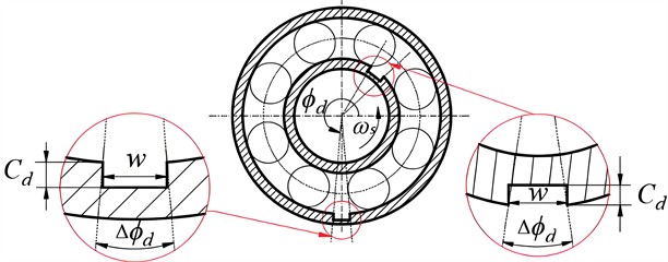
When a defect occurs in the inner ring, the additional deformation $δ (i)$ can be expressed as:

8

δ_{i} = \{\begin{array}{l} \frac{d}{2} - \sqrt{{(\frac{d}{2})}^{2} - {(\frac{w}{2})}^{2}}, & ω_{s} t + ϕ_{0} < φ_{j} < ω_{s} t + ϕ_{0} + Δ ϕ_{d}, \\ 0, & else, \end{array}

where $φ_{0}$ is the initial angular position of the defect. The total deformation caused by the inner ring fault is $δ = δ_{j} + δ_{i}$ .

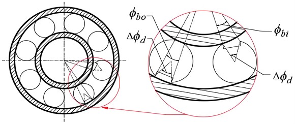
When a defect occurs in the rolling element, during one complete rotation cycle, it will contact both the inner and outer rings, generating additional deformation at each contact. The defect in the rolling element is illustrated in Fig. 2.

Assuming that the rolling element with a defect rotates at the same speed at any position, the angular position of the defect $φ_{s}$ can be expressed as:

9

\begin{array}{r} ϕ_{s} = \frac{ω_{s} D}{2 d} (1 - {(\frac{d}{D} c o s α)}^{2}) t + ϕ_{0} \end{array} .

The additional deformation $δ_{r}$ caused by the defect in the rolling element can be expressed as:

10

δ_{r} = \{\begin{array}{l} \frac{d}{2} - \sqrt{{(\frac{d}{2})}^{2} - {(\frac{w}{2})}^{2}} - (\frac{D_{o}}{2} - \sqrt{{(\frac{D_{o}}{2})}^{2} - {(\frac{w}{2})}^{2}}), & 0 < ϕ_{s} < ϕ_{b o}, \\ \frac{d}{2} - \sqrt{{(\frac{d}{2})}^{2} - {(\frac{w}{2})}^{2}} + (\frac{D_{i}}{2} - \sqrt{{(\frac{D_{i}}{2})}^{2} - {(\frac{w}{2})}^{2}}), & π < ϕ_{s} < π + ϕ_{b i}, \\ 0, & else, \end{array}

where $D_{o}$ is the diameter of the outer ring, $D_{i}$ is the diameter of the inner ring, and $ϕ_{b i}$ and $ϕ_{b 0}$ are the angular ranges of the defect when the rolling element contacts the inner and outer rings, respectively. The angular positions are given by $ϕ_{b i} = Δ ϕ_{d} d / D_{i}$ and $ϕ_{b o} = Δ ϕ_{d} d / D_{o}$ . In this case, the total deformation caused by the rolling element fault is $δ = δ_{j} + δ_{r}$ .

Fig. 2Schematic of a defect in the rolling element of the bearing

2.3. Development of rolling bearing simulation model

The development of a rolling bearing simulation model is primarily based on the actual parameters of a physical bearing. Operating conditions and defect parameters are set accordingly to accurately reflect the real operational state of the bearing. This section covers the construction of both the three-dimensional (3D) model and the dynamic model, with the overall framework illustrated in Fig. 3.

Fig. 3Framework of the rolling bearing simulation model

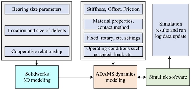
In this study, SolidWorks software is used to develop a three-dimensional (3D) model of the rolling bearing. The model is constructed based on the bearing’s dimensional parameters, the fit relationships between components, and different defect sizes at various locations. The model is then imported into ADAMS simulation software, where boundary conditions-including stiffness, friction coefficient, material properties, contact modes, rotational speed, and load-are defined. A co-simulation with Simulink is conducted to analyze the rolling bearing’s behavior and generate simulation data.

When defining the contact model for the bearing, it is necessary to establish contact interactions between the outer ring and rolling elements, rolling elements and the cage, as well as rolling elements and the inner ring to ensure accurate simulation results. Additionally, the contact mode between the inner surface of the outer ring and the rolling elements must be specified. The bearing system consists of 17 moving components, 2 fixed joints, 1 revolute joint, 13 planar joints, and 52 body-to-body contact interactions. During bearing operation, collisions occur, requiring the definition of contact forces between rolling elements and other components. These contact forces primarily consist of two components: elastic force, which arises when two objects come into contact and penetrate each other, and damping force, which results from velocity differences between components. ADAMS provides two methods for computing contact forces: the impact function method and the restitution coefficient method. Since the impact function method is easier to parameterize, it is adopted in this study [34].

The impact function is mathematically expressed as Eq. (11):

11

impact = \{\begin{array}{l} m a x (0, K {(x_{1} - x)}^{e} - s t e p (x, x_{1} - d, c_{m a x}, x_{1}, 0) * \dot{x}), & x < x_{1}, \\ 0, & x > x_{1}, \end{array}

where $x_{1}$ represents the reference distance between two components, $x$ is the actual distance, $\dot{x}$ denotes the relative impact velocity, $e$ is the deformation exponent, $K$ is the stiffness coefficient, $d$ is the reference penetration depth, and $c_{m a x}$ is the maximum damping coefficient when the penetration depth exceeds $d$ .

The function step, used for smoothing transitions, is defined as:

12

step = \{\begin{array}{l} h_{0}, & x < x_{0}, \\ h_{0} + (h_{1} - h_{0}) \frac{{(x - x_{0})}^{2}}{{(x_{1} - x_{0})}^{2}} [3 - \frac{2 (x - x_{0})}{x_{1} - x_{0}}], & x_{0} < x < x_{1}, \\ h_{1}, & x > x_{1} . \end{array}

The collision force is influenced by stiffness, deformation, relative velocity, maximum damping force, and the impact exponent. Additionally, relative motion generates friction forces, which must be appropriately defined. In setting up contact interactions, parametric variables must be established, including contact stiffness coefficient, force exponent, damping coefficient, penetration depth, Coulomb friction, static friction coefficient, dynamic friction coefficient, static friction transition velocity, and dynamic friction transition velocity. The contact stiffness and damping coefficients for rotating components are determined based on Hertz contact theory, with damping coefficients generally set between 0.1 % and 1 % of the contact stiffness [35].

In the actual installation of rolling bearings, the outer ring is fixed to the bearing housing, while the shaft drives the inner ring to rotate. The bearing studied in this paper is subjected to radial loads applied from top to bottom, with experimental loads of 300 N, 600 N, and 800 N. During the simulation, the load characteristics are modeled by applying a unidirectional force along the centerline of the inner ring’s axis. Additionally, the bearing is affected by its own gravitational force. To prevent sudden impacts, a gradually increasing driving force is applied, accelerating to the desired speed.

The ADAMS and Simulink are coupled for the joint simulation, as shown in Fig. 4. After obtaining the complete rolling bearing simulation model, the ADAMS/Controls module is used for integrated analysis.

To further evaluate the consistency between the measured and simulated signals, time-domain statistical indicators are analyzed. This study selects waveform indicators, impulse indicators, margin indicators, and kurtosis indicators for assessment. Their mathematical expressions are presented in Table 1.

Fig. 4Rolling bearing joint simulation process

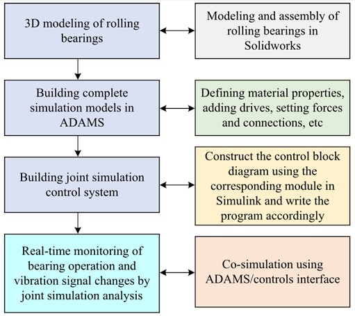
Table 1Time-domain statistical characterization

Waveform indicator	Pulse indicator	Amplitude indicator	Kurtosis indicator
$X_{W} = \frac{X_{m s s}}{\| \overline{X} \|}$	$X_{I} = \frac{X_{p e a k}}{\| \overline{X} \|}$	$X_{L} = \frac{X_{p e a k}}{X_{r}}$	$X_{K} = \frac{\frac{1}{N} \sum_{i = 1}^{N} x_{i}^{4}}{X_{m s}^{4}}$
Note: $X_{r m s}$ is the root mean square of the signal, $\| \overline{X} \|$ is the absolute mean of the signal, $X_{p e a k}$ peak is the peak of the signal, and $X_{r}$ is the square root amplitude of the signal

The waveform index characterizes the shape of the bearing vibration signal, while the impulse index quantifies the severity of impact within the signal. The margin index serves as an indicator of the fault severity, and the kurtosis index reflects the impact characteristics of the signal [36, 37].

To evaluate the consistency between measured and simulated signals, ten random segments, each containing 2,048 data points, the time-domain statistical features were computed for each segment and averaged. The calculated statistical indices for both measured and simulated signals, along with their relative deviations, are presented in Table 2.

The calculated relative deviations between the four time-domain statistical indicators of the simulation and measured data are small, with the maximum deviation being 6.56 % for the amplitude indicator of the rolling element signal. This deviation falls within a reasonable range, indicating that the simulated signal effectively replicates the measured signal. The causes of the relative deviation between the simulated and measured signals are as follows: (1) Random truncation of the signal introduces variability, which may increase the computational discrepancy between the simulated and measured signals; (2) The simulated signal represents only a subset of actual operating conditions, such as random sliding, cage clearance, specific clamping, and machining errors, all of which can influence the vibration signal measurements; (3) The measured signal is subject to strong noise interference, which further impacts the results.

When defects occur in rolling bearing components, their vibration signals undergo corresponding changes, which manifest in the frequency domain. Faults in different components correspond to distinct characteristic frequencies.

The fault frequency of the bearing can be calculated using the fault frequency formula [38], as shown in Table 3. In the table, $d$ is the ball diameter, $D$ is the center diameter, $Z$ is the number of balls, and $f_{r}$ is the frequency.

Table 2Calculated values of time-domain statistical indicators for measured and simulated signals and their relative deviations

Defect location	Type	Waveform indicator	Pulse indicator	Amplitude indicator	Kurtosis indicator
Normal	Measured	1.247	5.182	6.728	2.812
	Simulated	1.263	4.951	6.512	2.904
	Relative deviation (%)	1.28	4.46	3.21	3.27
Inner ring	Measured	1.548	11.742	15.861	7.118
	Simulated	1.589	11.368	15.434	7.297
	Relative Deviation (%)	2.65	3.19	2.70	2.51
Outer ring	Measured	1.305	9.567	11.582	3.216
	Simulated	1.273	9.128	10.874	3.051
	Relative deviation (%)	2.45	4.59	6.11	5.13
Rolling element	Measured	1.412	10.136	13.215	7.902
	Simulated	1.438	9.471	12.742	7.622
	Relative Deviation (%)	1.84	6.56	3.58	3.54

Table 3Bearing fault frequency equation

Fault condition	Fault pass frequency
Rolling element fault via outer race	$f_{o} = \frac{Z}{2} (1 - \frac{d}{D} c o s α) f_{r}$
Rolling element fault via inner race	$f_{i} = \frac{Z}{2} (1 + \frac{d}{D} c o s α) f_{r}$
Rolling element fault characteristic frequency	$f_{b} = \frac{D}{d} [1 - (\frac{d}{D} c o s α)] f_{r}$

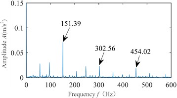
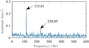
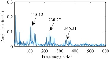
Based on the bearing fault frequency formulas, the calculated fault pass frequencies are 108.05 Hz for the outer race, 151.95 Hz for the inner race, and 115.08 Hz for the rolling element rotational frequency. The characteristic frequency distributions of the simulated sample in the frequency domain exhibit slight differences when compared to the measured sample. However, the distributions are very similar, as shown in Fig. 5.

By analyzing the envelope spectra of the measured and simulated signals shown in Fig. 5, it can be observed that the fault frequencies for the outer race in the measured and simulated signals are 108.35 Hz and 108.01 Hz, respectively. The fault frequencies for the inner race are 152.23 Hz and 151.39 Hz, and the rolling element fault frequencies are 115.01 Hz and 115.12 Hz. The relative deviations from the theoretical values are minimal.

However, slight differences in amplitude and fault frequency can still be observed between the measured and simulated signals. These discrepancies can be attributed to the differences between the simulation model and the actual field test environment. The field environment is influenced by many factors, some of which introduce errors relative to the set values. These factors include random sliding, lubrication conditions, external noise, and the influence of adjacent mechanical systems, all of which contribute to the differences between the simulation and the measured signals.

For bearing fault signals, simply analyzing the time-domain statistical features and frequency-domain envelope spectra does not fully reveal the similarities and differences between the measured and simulated signals. Additionally, the size of the bearing defects can also affect the energy peaks. Time-frequency analysis can combine frequency and time, allowing for the observation of signal frequency variations over different time periods [39].

Fig. 5Measured and simulated signal envelope spectra of rolling bearings

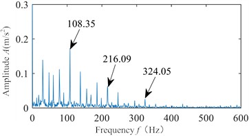
a) Measured signal envelope spectrum of the outer ring

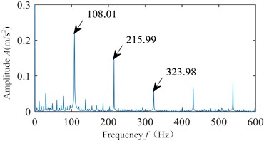
b) Simulated signal envelope of outer ring

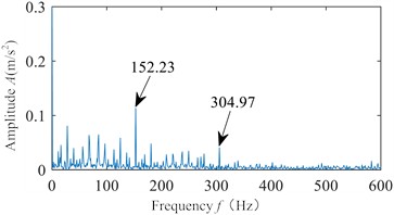
c) Measured signal envelope of inner ring

d) Simulated signal envelope of inner ring

e) Measured signal envelope of rolling element

f) Simulated signal envelope of rolling body

Wavelet transform was applied separately to both the measured and simulated data, using the cmor2-1 wavelet as the basis function, resulting in the time-frequency plots shown in Fig. 5. The distribution of vibration response energy in both the time and frequency domains can be clearly observed. In the measured data, excessive noise causes the energy to be more dispersed compared to the simulated signal, where the energy is more concentrated. The maximum energy is observed when the rolling element passes over the defect. The inner race and rolling element faults exhibit a distinct “double impact” phenomenon [41, 41].

In traditional neural network methods, it is assumed that the probability distributions of different datasets are consistent. However, in reality, due to the differences between the simulation model and the actual field conditions, the probability distributions of the simulated and measured fault-bearing signal datasets are not identical. The probability density of different signals reflects the likelihood of the signal falling within various amplitude ranges. By comparing the distribution of measured and simulated signals across different ranges, faults and anomalies can be more effectively identified. This study utilizes probability density comparison to analyze the consistency between simulated and measured signals. The probability density function is given by Eq. (13):

13

\begin{array}{r} P x = \underset{Δ x \to 0}{l i m} \frac{P [x < x (i) < x + Δ x]}{Δ x} \end{array},

where $x (i)$ represents the vibration signal amplitude that falls within the interval $x$ and $x + Δ x$ .

From the probability density distribution of the bearing under different health conditions, it can be observed that the simulated and measured data for the healthy bearing are highly similar. However, for the faulty bearings, there are noticeable differences between the simulated and measured data, with the simulated signal exhibiting higher probability density values. This discrepancy arises because, during actual operation, faulty bearings are influenced by various random factors, causing the probability distribution of the measured signal to be smoother, with lower probability density values.

This section first analyzes the failure modes of rolling bearings and explains the causes of vibration. Then, a bearing simulation model is developed based on the bearing parameters, and a coupled simulation is performed using ADAMS and Simulink software to generate the bearing simulation signals. Finally, to verify the generation of high-fidelity bearing simulation signals, a comparative analysis of the measured and simulated signals is conducted in terms of time-domain, frequency-domain, time-frequency analysis, and probability density distribution. This analysis ensures the validity of the generated simulation signals and provides comprehensive data support for neural network-based fault diagnosis of rolling bearings.

3. Simulation data-driven transfer diagnosis model

This study employs a model-parameter-based transfer learning approach, where simulation data of rolling bearings under various operating conditions or defect sizes are obtained through a simulation model to pre-train a weighted autoencoder model. The trained model parameters are then transferred and applied to the target domain dataset for analysis, enabling the assessment of bearing health. This approach not only demonstrates the feasibility of simulation data but also validates the model’s generalization performance. The specific model is shown in Fig. 6.

Fig. 6Schematic of defects in the inner and outer rings of the bearing

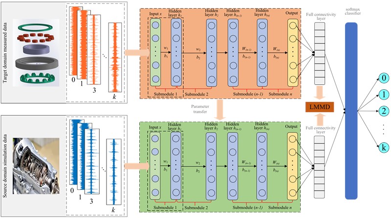
In the proposed weighted autoencoder, the self-attention mechanism functions as a feature dependency modeling module, calculating pairwise relationships among latent features to capture their contextual relevance. It outputs attention coefficients that indicate the relative importance of each feature dimension. The weight allocation mechanism, on the other hand, acts as a feature reweighting and aggregation module. Guided by the attention scores, it quantitatively adjusts the amplitude of each feature, amplifying those that contribute more significantly to fault identification and suppressing redundant or noise-sensitive ones. Therefore, the two mechanisms work in tandem: the self-attention mechanism determines which features are important by learning dependencies, while the weight allocation mechanism decides how much each feature contributes to the final latent representation. This design ensures adaptive enhancement of fault-relevant information and improves the robustness and transferability of extracted features.

To address the similarity problem between the source domain and the target domain and minimize their distributional distance, many researchers employ Maximum Mean Discrepancy (MMD) to measure the distributional discrepancy between the two domains. The primary advantage of MMD is its independence from class labels, as it measures the distance based solely on the distribution of hidden features. MMD maps the source and target domain data into a Reproducing Kernel Hilbert Space (RKHS), representing them as the inner product of two points in a high-dimensional space. The distributional distance in this space can be measured using Eq. (14), which quantifies the distance between the distributions $D_{S}$ and $D_{T}$ :

14

\begin{array}{r} M M D^{2} (D_{S}, D_{T}) = {‖\frac{1}{n_{s}} \sum_{i = 1}^{n_{s}} f (x_{i}) - \frac{1}{n_{t}} \sum_{j = 1}^{n_{t}} f (x_{j})‖}_{H}^{2} \end{array},

where in this equation, $x_{i}$ and $x_{j}$ are data samples from $D_{S}$ and $D_{T}$ , respectively; $n_{s}$ and $n_{t}$ denote the number of samples in $D_{S}$ and $D_{T}$ ; $f (\cdot)$ is the mapping function; and $H$ represents the Reproducing Kernel Hilbert Space.

The key to MMD lies in the selection of the mapping function. The most commonly used functions include Gaussian and linear kernels. However, the exact kernel function is typically unknown, requiring decomposition, which can be expressed as Eq. (15):

15

\begin{array}{r} M M D (D_{s}, D_{T}) = \frac{1}{n_{s}^{2}} \sum_{i = 1}^{n_{s}} \sum_{j = 1}^{n_{s}} k (z_{i}^{s}, z_{j}^{s}) - \frac{1}{n_{s} n_{t}} \sum_{i = 1}^{n_{s}} \sum_{j = 1}^{n_{t}} k (z_{i}^{s}, z_{j}^{t}) + \frac{1}{n_{t}^{2}} \sum_{i = 1}^{n_{t}} \sum_{j = 1}^{n_{t}} k (z_{i}^{t}, z_{j}^{t}) \end{array} .

The Gaussian kernel function enables mapping data into an infinite-dimensional space and can be defined as:

16

\begin{array}{r} k (x_{1}, x_{2}) = e x p (- {∥x_{1} - x_{2}∥}^{2} / (2 γ^{2})) \end{array},

where $γ$ represents the bandwidth parameter.

While MMD effectively aligns the global distributions of the source and target domains, it neglects the alignment of different fault types within each subdomain, which may lead to misclassification of marginal distribution data. To address this limitation, LMMD is introduced to achieve both subdomain and global alignment. LMMD assigns weights to each sample based on its category, reducing distributional differences through weight calculation, as shown in Eq. (17):

17

L M M D (D_{s}, D_{T}) = \frac{1}{C} \sum_{c = 1}^{c} {∥\sum_{x_{i}^{s} \in D_{s}} ω_{i}^{s c} f (x_{i}^{s}) - \sum_{x_{j}^{s} \in D_{T}} ω_{j}^{t c} f (x_{j}^{t})∥}_{H}^{2}

= \frac{1}{C} \sum_{c = 1}^{c} [\sum_{i = 1}^{n_{s}} \sum_{j = 1}^{n_{s}} ω_{i}^{s c} ω_{j}^{s c} k (z_{i}^{s}, z_{j}^{s}) - 2 \sum_{i = 1}^{n_{s}} \sum_{j = 1}^{n_{t}} ω_{i}^{s c} ω_{j}^{s c} k (z_{i}^{s}, z_{j}^{t}) + \sum_{i = 1}^{n_{t}} \sum_{j = 1}^{n_{t}} ω_{i}^{t c} ω_{j}^{t c} k (z_{i}^{t}, z_{j}^{t})],

where $C$ denotes the number of fault categories, and $ω_{i}^{s c}$ and $ω_{j}^{t c}$ represent the weights of the $i$ -th sample in $D_{S}$ and the $j$ -th sample in $D_{T}$ within category $c$ . These weights can be computed using Eq. (18):

18

\begin{array}{r} ω_{i}^{c} = \frac{y_{i c}}{\sum_{(x_{j}, y_{j}) \in D} y_{j c}}, \end{array}

where $\sum_{(x_{j} y_{j}) = D} y_{j c}$ represents the total sum of samples belonging to category $c$ , and $y_{i c}$ is the $c$ -th element of the label vector $y_{i}$ .

The pretraining process of the network involves feeding source domain data into a weighted autoencoder network, where the training objective is to minimize the classification loss of the source domain using a cross-entropy loss function $L_{c}$ . In the transfer learning stage, after iterative training, the cross-entropy loss of the source domain is minimized, and the objective shifts to reducing the distribution discrepancy between the two domains, which is expressed as $L_{L M M D}$ . The final training objective is formulated as a joint loss function combining cross-entropy loss and LMMD, as shown in Eq. (19):

19

\begin{array}{r} m i n \{L_{c} + λ L_{L M M D}\} \end{array},

where $λ$ is a trade-off parameter selected through extensive experiments from the set 0.01, 0.05, 0.1, 0.5, 1,5, 10, 50, with the optimal value determined to be 0.5.

Once the distributional difference is sufficiently reduced, the model is capable of accurately classifying both source and target domain data. LMMD is primarily applied in the fully connected layer to measure the domain differences, and network parameters are updated through backpropagation. The trained model then utilizes a Softmax classifier to output classification results:

The detailed transfer diagnosis process is illustrated in Fig. 7.

Fig. 7Rolling bearing transfer learning fault diagnosis flowchart

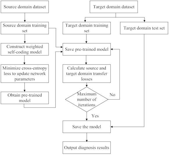
The simulation data is utilized as the source domain dataset for pretraining a weighted autoencoder model. The network parameters are updated by minimizing the classification loss using the cross-entropy loss function, ultimately yielding a pretrained network model. Subsequently, the transfer loss is computed based on both the source domain and target domain training sets. Once the maximum number of iterations is reached, the model is saved. Finally, the trained model is applied to the target domain test set for rolling bearing fault diagnosis.

4. Transfer diagnosis across different operating conditions

In certain real-world scenarios, acquiring fault measurement data for bearings is challenging and costly. To address this issue, a modeling approach can be employed to generate bearing datasets for fault diagnosis. However, a critical challenge lies in determining whether the constructed model is applicable to solving such problems. Therefore, in this section, a simulation model is utilized to generate high-fidelity data under different operating conditions for model training. The trained model is then validated using real measurement data, enabling transfer learning across different operating conditions and verifying the feasibility of the proposed transfer diagnosis model.

4.1. Description of transfer datasets across different operating conditions

For bearing data transfer between different operating conditions, two types of variations are considered: one with a fixed rotational speed and varying load, and the other with a fixed load and varying rotational speed. In each case, 10 different types of bearing health conditions are established, including normal, outer ring fault, inner ring fault, and rolling element fault. Each fault type is further categorized based on defect sizes of 0.2 mm, 0.6 mm, and 1.0 mm. The detailed dataset specifications are presented in Tables 4 and 5.

Table 4Simulation-actual measurement of transfer task design between different rotational speeds

Task ID	Fixed load	Transfer paths	Source domain samples	Target domain samples
3-3		Simulation-actual measurement
A1	30 KG	(500 r/min)-(800 r/min)	4000	4000
A2		(500 r/min)-(1200 r/min)	4000	4000
A3		(800 r/min)-(500 r/min)	4000	4000
A4		(800 r/min)-(1200 r/min)	4000	4000
A5		(1200 r/min)-(500 r/min)	4000	4000
A6		(1200 r/min)-(800 r/min)	4000	4000

Table 5Simulation-actual measurement of transfer task design between different loads

Task ID	Fixed rotational speed	Transfer paths	Source domain samples	Target domain samples
3-3		Simulation-actual measurement
B1	1200 r/min	(30 KG)-(60 KG)	4000	4000
B2		(30 KG)-(80 KG)	4000	4000
B3		(60 KG)-(30 KG)	4000	4000
B4		(60 KG)-(80 KG)	4000	4000
B5		(80 KG)-(30 KG)	4000	4000
B6		(80 KG)-(60 KG)	4000	4000

As shown in Table 4, for transfer learning across different rotational speeds, the load was fixed at 30 kg, while three rotational speeds were considered: 500 r/min, 800 r/min, and 1200 r/min. Six transfer tasks (A1-A6) were designed, with the transfer path primarily involving simulation data as the source domain and experimental data as the target domain. Each operating condition was divided into samples of 1,024 data points, with 400 samples per condition. The source domain dataset contained 4,000 samples, and the target domain dataset also contained 4,000 samples. The datasets were split into training and testing sets in a 7:3 ratio to ensure robust model evaluation.

As shown in Table 5, for transfer learning across different load conditions, the rotational speed was fixed at 1200 r/min, while three load levels were considered: 30 kg, 60 kg, and 80 kg. Six transfer tasks (B1-B6) were designed, with the transfer process involving transfer from simulation data as the source domain to experimental data as the target domain. Both the source and target domain datasets contained 4,000 samples each. The sample acquisition process and dataset partitioning followed the same methodology as described in Table 4.

4.2. Experimental results analysis and discussion of model transfer

In this paper, classification accuracy was adopted as the main evaluation index to measure the model performance under different transfer tasks. In addition to accuracy, the supplementary indicator – $F 1$ -score – is also introduced to comprehensively evaluate model performance. The metric can provide a more balanced view, particularly when class imbalance may exist in practical applications. The $F 1$ score is defined as follows:

20

\begin{array}{r} F 1 = \frac{2 P R}{P + R} \end{array}, P = \frac{T P}{T P + F P}, R = \frac{T P}{T P + F N},

where, $P$ , $R$ , $T P$ , $F P$ , and $F N$ represent the precision, recall, true positives, false positives, and false negatives, respectively. The $F 1$ -score, as the harmonic mean of precision and recall, reflects both sensitivity and specificity of the classification model. In subsequent calculations, all the $F 1$ -score metrics are calculated on a per-class basis and then averaged using the macro-average strategy to ensure equal weight for each fault category. The results are obtained from the same test sets used for accuracy evaluation.

In subsequent experiments, we conducted thorough comparative tests against mainstream SAE, SDAE, and VAE models. Key parameter configurations for the comparative experiments are summarized in Table 6.

Table 6Experimental parameter settings

Category		Parameter setting
Simulation data generation	Rotational speeds	600, 900, 1200, 1500, 1800 r/min
	Loads	0.5, 1.0, 1.5, 2.0, 2.5 kN
	Fault types	Inner ring, outer ring, rolling element
	Fault sizes	0.3 mm, 0.6 mm, 0.9 mm
Feature extractor (Proposed)	Encoder type	Attention-assisted weighted autoencoder
	Input dimension	1024 (time-domain samples)
	Hidden layers	[512, 256, 128]
	Attention heads	4
	Dropout	0.3
Transfer adaptor (LMMD)	Kernel type	Gaussian RBF
	Number of subdomains	5
	Trade-off parameter $λ$	0.5
Training setup	Optimizer	Adam
	Initial learning rate	0.001
	Batch size	128
	Epochs	100
	Early stopping	patience = 10
Noise robustness test	SNR levels	–5 dB, –10 dB, –15 dB
	Noise type	Gaussian white noise
	Metric	Transfer accuracy (%)

The target domain data from different rotational speed transfer tasks were fed into the model for evaluation. Each experiment was run 10 times, and the average results were recorded. To assess performance, the proposed model was compared with SAE, SDAE, and VAE. The results are illustrated in Fig. 8, while the transfer accuracy is presented in Table 7.

From Fig. 8, it can be observed that transferring simulation data collected under different rotational speeds to measured data yields consistently higher diagnostic accuracy when using the proposed model compared with SAE, SDAE, and VAE. According to Table 7, the average accuracy across six transfer tasks for SAE, SDAE, VAE, and the proposed method is 87.99 %, 90.87 %, 91.43 %, and 96.76 %, respectively, with SAE yielding the lowest transfer diagnostic performance. Additionally, our method obtain the highest $F 1$ -score. This indicates that the proposed attention-assisted weighted autoencoder effectively enhances the representation of fault-related features and improves cross-speed transferability. The key reason lies in the encoder’s attention mechanism, which adaptively assigns higher weights to vibration features that contribute more significantly to fault discrimination while suppressing redundant or condition-specific information. As a result, the learned latent space becomes both more compact and more discriminative, ensuring that the domain discrepancy between simulated and measured data is reduced at the feature level. Furthermore, by jointly optimizing the reconstruction and transfer objectives, the encoder learns features that preserve the physical interpretability of the original vibration responses while remaining invariant to speed variations. This dual constraint effectively mitigates the negative transfer effect commonly observed in shallow autoencoders, where irrelevant speed-dependent features dominate the learned representation. Therefore, the superior performance across different speeds confirms that the attention mechanism enables selective knowledge transfer from simulated to real environments.

Fig. 8Comparison of transfer methods between different rotational speeds

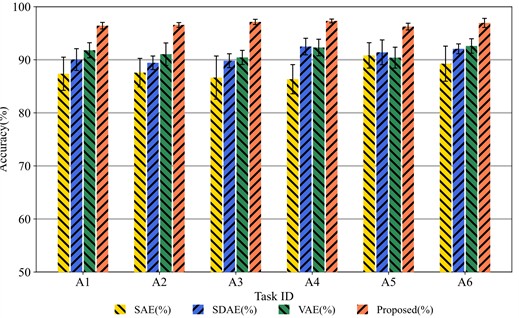
Table 7Transfer accuracy of different methods between different speeds (%)

Task ID	SAE	SDAE	VAE	Proposed
A1	87.36±3.13	90.04±2.05	91.79±1.42	96.42±0.62
A2	87.57±2.69	89.43±1.28	91.05±2.12	96.56±0.45
A3	86.64±4.07	89.82±1.31	90.44±1.33	97.13±0.49
A4	86.34±2.75	92.49±1.56	92.31±1.56	97.31±0.36
A5	90.82±2.40	91.40±2.34	90.4±1.97	96.25±0.64
A6	89.26±3.31	92.06±0.93	92.6±1.36	96.94±0.86
$F 1$	0.901	0.943	0.948	0.984

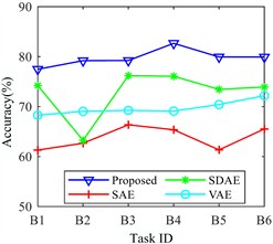
The diagnostic results for different models using test data from varying load conditions are presented in Fig. 9.

As illustrated in Fig. 9, the SAE method exhibits the lowest transfer performance, whereas the proposed approach achieves significantly higher fault identification accuracy. The diagnostic accuracy and $F 1$ -score presented in Table 8 further confirms that when using different load conditions for transfer learning, the performance of SAE, SDAE, and VAE remains relatively low, with marginal differences among these methods. In contrast, the proposed method demonstrates a substantial improvement in transfer diagnostic performance. The average accuracy across the six transfer tasks (B1-B6) reaches 96.73 %, surpassing the other three methods.

Fig. 9Comparison of transfer methods between different loads

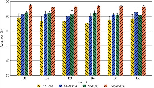
Table 8Transfer accuracy of different methods between loads (%)

Task ID	SAE	SDAE	VAE	Proposed
B1	89.03 ± 2.67	91.22 ± 1.05	92.45 ± 0.89	97.45 ± 0.55
B2	86.84 ± 3.25	91.71 ± 1.74	92.04 ± 1.23	96.20 ± 0.63
B3	86.68 ± 4.10	90.26 ± 1.35	91.16 ± 2.64	96.49 ± 0.47
B4	85.38 ± 3.51	90.13 ± 2.02	92.10 ± 1.62	97.05 ± 0.44
B5	87.45 ± 2.42	91.03 ± 1.09	90.93 ± 0.91	96.71 ± 0.34
B6	88.49 ± 2.65	92.64 ± 2.31	90.76 ± 2.15	96.49 ± 0.68
$F 1$	0.894	0.937	0.944	0.979

To further interpret these results, the following analysis discusses the underlying reasons for the observed performance differences. As shown in Tables 7-8, the proposed model achieves an average diagnostic accuracy of 96.73 %, which surpasses all compared models under different load transfer tasks. This improvement demonstrates that the LMMD-based alignment method provides a more effective strategy for mitigating distribution mismatch between domains with different mechanical loads. Unlike traditional global alignment metrics such as MMD or CORAL, LMMD decomposes the overall discrepancy into class-wise subdomain distances, ensuring that both global and local distributions are simultaneously aligned. This class-conditional alignment prevents the mixing of latent features belonging to different fault categories and thus reduces inter-class confusion during domain transfer. Moreover, the attention-weighted latent representation further enhances this process by concentrating the feature energy within fault-relevant subspaces. Consequently, LMMD can perform more precise alignment within those subspaces, leading to stable transfer performance even when the external load varies drastically. The smaller standard deviations reported in Table 11 also suggest that the proposed model achieves higher robustness and consistency compared to traditional MMD-based approaches.

As shown in Tables 7 and 8, the proposed attention-assisted weighted autoencoder achieves not only the highest classification accuracy but also the highest $F 1$ -score under both cross-speed and cross-load transfer conditions. This indicates that the model maintains an excellent balance between precision and recall, thereby demonstrating strong diagnostic robustness even under potential class imbalance. The improvement is mainly attributed to the attention-guided feature weighting and LMMD-based domain alignment, which enhance the discriminative and transferable representations of fault features.

To evaluate the noise robustness of the employed methods, Gaussian white noise with varying SNRs were added to different fault signals. The SNR is defined as follows:

21

\begin{array}{r} S N R_{d b} = 10 \times {l o g}_{10} \{\frac{P_{1}}{P_{2}}\} \end{array},

where $P_{1}$ represents the power of the original signal, and $P_{2}$ denotes the power of the noise signal. A higher SNR indicates lower noise interference.

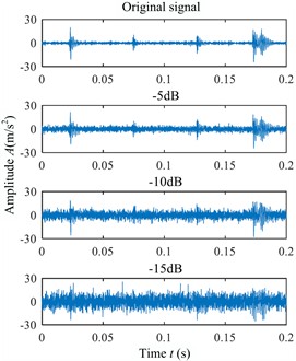
To comprehensively assess the impact of noise, Gaussian white noise with SNRs of –5 dB, –10 dB, and –15 dB was added to the datasets under different rotational speeds (Table 4) and varying loads (Table 5). For a more intuitive visualization, Fig. 10 illustrates the vibration signals of both simulated and measured data at a rotational speed of 1200 r/min with a defect size of 0.6 mm, encompassing inner ring, outer ring, and rolling element faults after incorporating noise levels of –5 dB, –10 dB, and –15 dB.

Fig. 10Measurement and simulation of vibration signals with different SNR at different defect sites

a) Inner ring simulation with different SNR signals

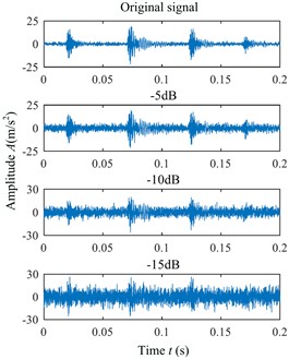
b) Simulated inner ring with different SNR signals

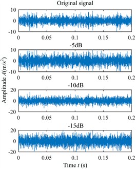
c) Outer ring measured with different SNR signals

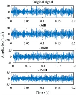
d) Outer ring simulation with different SNR signals

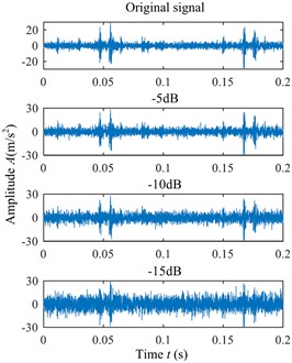
e) Rolling body measured with different SNR signals

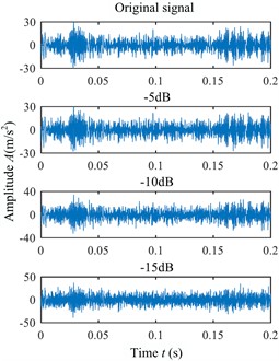
f) Rolling body simulation with different SNR signals

The datasets with different SNRs were subjected to transfer diagnosis according to the predefined transfer tasks, categorized as A1-A6 for varying rotational speeds and B1-B6 for different load conditions. The corresponding transfer results are presented in Fig. 11.

In Fig. 11, subfigures 11(a), 11(c), and 11(e) illustrate the transfer diagnosis experiments under different rotational speeds with varying levels of SNR noise interference, while subfigures 11(b), 11(d), and 11(f) present the transfer diagnosis experiments under different load conditions with added noise interference. Observing 11(a), 11(c), and 11(e) or 11(b), 11(d), and 11(f) individually reveals that as the SNR decreases, the noise signal becomes more dominant, masking the critical fault features of the rolling bearing and leading to reduced diagnostic accuracy. Under strong noise conditions (SNR = –10 dB and –15 dB), the proposed model maintains superior accuracy and lower standard deviation compared to other baselines. This demonstrates that the attention-weighted encoder not only enhances fault feature representation but also contributes to denoising through adaptive feature weighting, thereby improving robustness against environmental interference.

Fig. 11Comparison of different methods for adding noise with different SNRs under different operating conditions

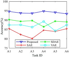
a) Diagnosis accuracy comparison of adding –5 dB noise disturbance at different speeds

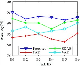
b) Diagnosis accuracy comparison of adding –5 dB Noise interference under different loads

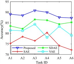
c) Diagnosis accuracy comparison of adding –10 dB at different speeds

d) Diagnosis accuracy comparison of adding –10 dB under different loads

e) Diagnosis accuracy comparison of adding –15 dB at different speeds

f) Diagnosis accuracy comparison of adding –15 dB at different loads

In practical machinery monitoring, signal contamination by environmental and electrical noise is inevitable, and thus robustness to low SNR scenarios is a crucial performance indicator. The proposed attention-assisted autoencoder contributes to noise resilience in two ways. First, the attention mechanism dynamically reweights latent features according to their relevance to fault characteristics, effectively filtering out noise components that exhibit low correlation with diagnostic patterns. Second, the joint reconstruction and LMMD objectives regularize the encoder to maintain structural consistency across domains, thereby avoiding overfitting to noise fluctuations. Compared with conventional denoising autoencoders that passively remove random noise through reconstruction loss, the attention mechanism provides an adaptive and feature-driven filtering process. As a result, the model not only achieves higher mean accuracy but also exhibits smaller performance degradation as SNR decreases. This robustness under severe noise demonstrates the practicality of the proposed approach for real-world fault diagnosis environments. Overall, the comparative analysis of noise robustness between the proposed method and SAE, SDAE, and VAE indicates that the proposed approach achieves superior transfer diagnosis performance, exhibiting significantly lower fluctuations than the other three methods. This validates the model’s generalization capability and resilience to noise interference. Besides, comparative experiments demonstrate that models incorporating both the self-attention and weight allocation mechanisms achieve higher diagnostic accuracy and better domain transfer performance than those using only one of them. The self-attention module captures feature correlations, while the weighting module quantitatively enhances discriminative features. This complementary design effectively suppresses noise and redundancy, maintaining robust performance even under low SNR conditions (e.g., –10 dB and –15 dB).

To further verify the generality and stability of the proposed approach, two additional sets of comparative experiments were conducted. The first set focused on evaluating the effect of employing more advanced feature extractors under the same LMMD adaptor, while the second set examined the impact of alternative transfer mechanisms when combined with the proposed attention-weighted feature extractor. These experiments are intended to validate that the observed improvements are not simply attributable to the baseline selection, but rather to the fundamental advantages of the proposed framework.

In this experiment, the LMMD adaptor was kept unchanged, while different feature extractors were employed, including SAE, SDAE, VAE, 1D-ResNet, TCN, Transformer encoder, and the proposed attention-weighted encoder. The results are illustrated in Fig. 12 (A1-A6), while Table 9 reports the transfer accuracies across six rotational speed transfer tasks. It can be observed that incorporating more powerful feature extractors such as ResNet, TCN, and Transformer significantly improves the baseline performance compared with shallow autoencoders. For instance, the average accuracy increased from 91.43 % (VAE) to 93.82 % (ResNet), 94.53 % (TCN), and 95.24 % (Transformer). Nevertheless, the proposed attention-weighted encoder still achieved the highest overall performance, with an average accuracy of 96.76 % and the lowest variance across tasks. This demonstrates that the effectiveness of the proposed model does not rely on weaker baselines; even when compared against modern, high-capacity architectures under identical transfer conditions, the proposed feature reweighting mechanism continues to provide clear improvements in both accuracy and stability. These findings confirm that the attention mechanism successfully enhances the discriminative power of fault-related features and reduces redundancy, thereby complementing rather than duplicating the advantages of advanced backbone networks.

Fig. 12Comparison of transfer methods between different rotational speeds

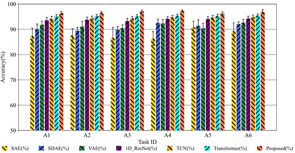
Table 9Transfer accuracy of different methods between different speeds (%)

Task ID	SAE	SDAE	VAE	1D-ResNet	TCN	Transformer	Proposed
A1	87.36±3.13	90.04±2.05	91.79±1.42	93.52±1.11	94.15±0.95	95.08±0.77	96.42±0.62
A2	87.57±2.69	89.43±1.28	91.05±2.12	93.76±1.08	94.40±0.83	95.22±0.65	96.56±0.45
A3	86.64±4.07	89.82±1.31	90.44±1.33	93.25±1.12	94.30±0.79	95.11±0.70	97.13±0.49
A4	86.34±2.75	92.49±1.56	92.31±1.56	94.12±0.88	94.78±0.74	95.36±0.62	97.31±0.36
A5	90.82±2.40	91.40±2.34	90.40±1.97	94.05±0.97	94.69±0.81	95.28±0.68	96.25±0.64
A6	89.26±3.31	92.06±0.93	92.60±1.36	94.22±0.95	94.85±0.77	95.41±0.66	96.94±0.86

To isolate the effect of the transfer mechanism, we fixed the feature extractor to the proposed attention-weighted encoder and replaced the LMMD adaptor with three representative alternatives: CORAL, DANN, and JAN. The results of six load transfer tasks (B1-B6) are illustrated in Fig. 13 and the diagnostic accuracy are summarized in Table 10. It can be observed that all transfer mechanisms improved diagnostic accuracy compared with training without adaptation, but clear performance differences emerged. CORAL achieved an average accuracy of 93.87 %, DANN further improved to 94.85 %, and JAN reached 95.32 %. The LMMD adaptor, however, delivered the highest accuracy of 96.73 % with the smallest variance. These results confirm that although adversarial or correlation-based alignment methods are capable of reducing global distributional discrepancies, they are less effective in simultaneously addressing local sub-domain misalignments, which often arise in cross-condition and cross-location scenarios. By synchronously aligning both global and sub-domain distributions, LMMD better mitigates inter-condition bias, thereby enhancing robustness under severe distribution shifts. This validates the necessity of employing LMMD as the alignment module in the proposed framework.

Fig. 13Comparison of different transfer mechanisms between different loads

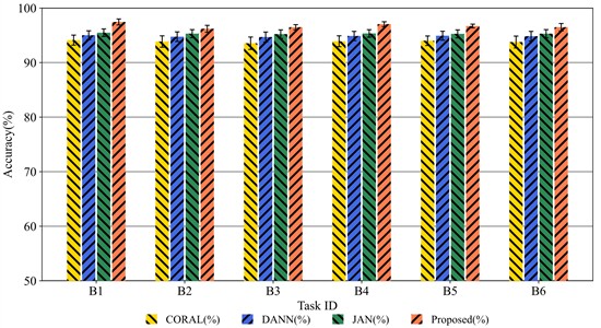
Table 10Transfer accuracy of different transfer mechanisms with the proposed feature extractor (%)

Task ID	CORAL	DANN	JAN	Proposed
B1	94.12±0.92	95.02±0.81	95.48±0.70	97.45±0.55
B2	93.86±1.05	94.75±0.88	95.31±0.74	96.20±0.63
B3	93.55±1.14	94.69±0.91	95.22±0.78	96.49±0.47
B4	93.92±1.00	94.88±0.85	95.35±0.69	97.05±0.44
B5	94.01±0.87	94.93±0.82	95.27±0.73	96.71±0.34
B6	93.77±1.09	94.84±0.89	95.30±0.75	96.49±0.68

Overall, the extended experiments with advanced feature extractors and alternative transfer mechanisms consistently demonstrate that the superior performance of the proposed approach cannot be solely attributed to baseline limitations. Instead, the improvements originate from the synergy between the simulation data-driven augmentation, the attention-assisted feature weighting, and the LMMD-based distribution alignment. These components jointly contribute to the robustness and generalization capability of the proposed model, enabling reliable cross-condition and cross-location fault diagnosis even under strong noise disturbances.

5. Transfer diagnosis using reconstructed data from different locations

Due to significant differences in the installation environments, the vibration frequency and amplitude of bearing signals collected from the same device and bearing model may vary. Additionally, the external environmental influences can further impact the data collection process. In some harsh environmental conditions, it may be difficult to install sensors on the bearing, making it impossible to gather corresponding fault data. Therefore, it is essential to consider using bearing data collected from different locations of the same device for fault diagnosis.

5.1. Description of transfer datasets from different locations

As shown in the bearing fault data collection experimental setup in Fig. 14, data collected from different locations on the bearing, including the far-end, fault-end, and near-ground positions, are used for diagnosis. In this study, the fault-end position is considered the location where the faulty bearing is installed. Simulation data is used to train the model, and test data is obtained from the far-end position, which is distant from the faulty bearing installation. The specific transfer tasks are shown in Tables 11 and 12.

Fig. 14Fault diagnosis test bench

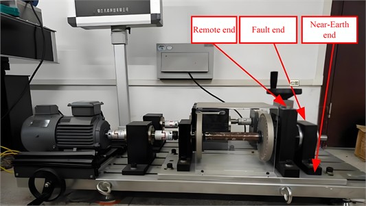
Table 11Transfer diagnosis between different positions and speeds

Task ID	Fixed condition	Transfer paths	Source domain samples	Target domain samples
3-3		Simulation (fault end) - Real measurement (remote end)
C1	30 KG	(500 r/min)-(500 r/min)	4000	4000
C2		(800 r/min)-(800 r/min)	4000	4000
C3		(1200 r/min)-(1200 r/min)	4000	4000
C4		(1500 r/min)-(1500 r/min)	4000	4000

Table 12Transfer diagnosis between different positions and loads

Task ID	Fixed condition	Transfer paths	Source domain samples	Target domain samples
3-3		Simulation (fault end) - real measurement (remote end)
D1	1200 r/min	(0 KG)-(0 KG)	4000	4000
D2		(30 KG)-(30 KG)	4000	4000
D3		(60 KG)-(60 KG)	4000	4000
D4		(80 KG)-(80 KG)	4000	4000

For the transfer between different locations, a fixed load of 30KG and four different speeds-500r/min, 800r/min, 1200r/min, and 1500r/min-are selected. The transfer is conducted from the fault-end simulation data to the far-end measured data. The Task IDs are set as C1 to C4. Sample acquisition and dataset partitioning follow the same approach as in Section 4.1 for transfer between different operating conditions.

In addition to setting the speed variation, four different loads – 0 KG, 30 KG, 60 KG, and 80 KG – are used for transfer tasks, with a fixed operating condition of 1200 r/min. These tasks are assigned the transfer Task IDs D1 to D4. The number of samples for both the source and target domains is set to 4000, and the sample partitioning follows the same method as described in Table 11.

5.2. Transfer results analysis

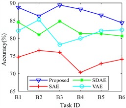
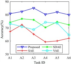
The transfer tasks constructed in Tables 11 and 12 are input into the built model for training and testing. The results are then compared with those from the SAE, SDAE, and VAE methods. When using fixed load conditions, with the source domain being fault-end simulation data and the target domain being remote-end real measurement data for transfer tasks C1 to C4, the experiment is run 10 times and the average result is taken. The results are shown in Fig. 15, and the average diagnostic accuracy is provided in Table 13. When using fixed speed conditions and Task IDs D1 to D4 for transfer diagnosis, the results are shown in Fig. 16, and the average diagnostic accuracy is provided in Table 14.

Fig. 15Transfer comparison of rotational speed between different positions

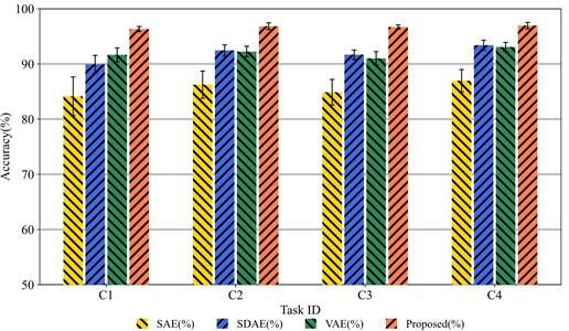
Table 13Transfer diagnostics accuracy of different methods between rotational speeds at different locations (%)

Task ID	SAE	SDAE	VAE	Proposed
C1	84.13±3.52	89.93±1.62	91.65±1.26	96.32±0.46
C2	86.24±2.48	92.46±1.01	92.24±0.97	96.83±0.62
C3	84.88±2.33	91.68±0.85	91.01±1.22	96.69±0.39
C4	86.95±2.04	93.40±0.91	93.07±0.83	96.95±0.58

As shown in Fig. 15 and Table 13, for the migration between different positions with fixed load, the proposed method achieves a higher accuracy across the four corresponding speeds. The average accuracy reaches 96.69%, indicating that the model exhibits strong generalization ability. In contrast, the results using SAE, SDAE, and VAE for migration diagnosis are relatively poor, with SAE performing the worst and exhibiting the largest fluctuation in diagnostic accuracy.

Using constant speed and migrating between different positions with four corresponding loads, migration tasks D1 to D4 were set. As shown in Fig. 16, the migration comparison for different loads and the corresponding average migration diagnostic accuracy in Table 14, after migration, the proposed method achieves an average accuracy of 96.53 %. The other three methods show considerable fluctuation and poor robustness. Thus, the proposed migration diagnostic model demonstrates a clear diagnostic advantage over the other three methods.

Table 14Transfer diagnostics accuracy of different methods between loads at different locations (%)

Task ID	SAE	SDAE	VAE	Proposed
D1	88.31±2.55	92.36±1.48	91.64±0.98	96.17±0.72
D2	86.57±3.81	91.06±1.63	90.43±1.16	95.86±0.42
D3	85.39±2.86	92.58±1.14	91.80±0.89	96.73±0.28
D4	86.27±1.94	90.34±0.94	91.04±1.33	97.35±0.56

Following the procedure in Section 4, where simulation and real measurement data for different operating conditions were added with noise at different SNRs, the same process was performed for the migration datasets between different positions to test the model’s resistance to interference. The specific diagnostic results are shown in Tables 15 and 16.

Fig. 16Transfer comparison of load between different positions

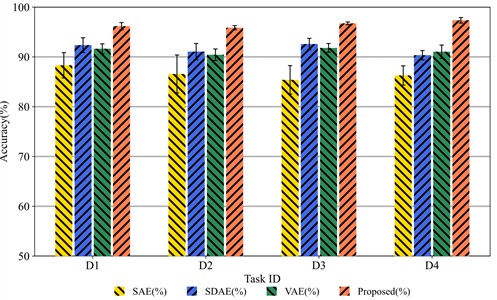
Table 15Transfer diagnostic accuracy (%) of rotational speed between positions with different SNR noises added

SNR (dB)	Methods	C1	C2	C3	C4
–5	Proposed	93.74	95.05	92.62	92.86
	SAE	79.27	81.01	83.76	80.43
	SDAE	89.23	87.45	86.07	88.40
	VAE	85.77	85.06	87.82	84.24
–10	Proposed	87.38	90.29	88.61	88.08
	SAE	72.45	72.36	78.63	75.20
	SDAE	83.54	86.50	84.48	85.17
	VAE	80.25	80.96	83.14	83.02
–15	Proposed	81.34	79.29	82.06	80.91
	SAE	54.26	63.85	62.59	62.72
	SDAE	74.33	72.13	74.58	76.04
	VAE	71.24	69.79	62.57	68.04

Table 16Transfer diagnostic accuracy (%) of load between positions with different SNR noises added

SNR (dB)	Methods	D1	D2	D3	D4
–5	Proposed	94.14	92.07	93.45	94.61
	SAE	83.96	83.42	81.88	84.58
	SDAE	90.06	91.30	85.70	88.62
	VAE	89.03	88.35	83.65	86.04
–10	Proposed	84.35	86.50	87.92	88.04
	SAE	74.26	70.33	70.57	72.86
	SDAE	83.07	80.55	83.70	82.81
	VAE	81.30	82.06	84.03	79.58
–15	Proposed	76.20	79.35	80.31	79.03
	SAE	62.04	66.44	61.07	59.85
	SDAE	72.69	70.52	68.82	67.49
	VAE	71.08	73.56	72.63	70.71

For the noise resistance test on migration between different positions, Gaussian white noise with SNRs of –5 dB, –10 dB, and –15 dB was added to the simulation and real measurement data for each condition in tasks C1 to C4 and D1 to D4. The noisy datasets were then used for migration diagnostics in the model, and the results are shown in Tables 15 and 16. The proposed method demonstrates high diagnostic accuracy. Although the diagnostic accuracy decreases with the increase in noise intensity, the drop is less pronounced compared to the other three methods, with smaller fluctuations and better robustness. This indicates that the model has better noise resistance compared to the other methods.

5.3. Summary and discussion

The comprehensive experiments conducted across various transfer scenarios – including changes in speed, load, and sensor location – collectively validate the generalization capability of the proposed approach. The results consistently demonstrate that the combination of simulation-driven data augmentation, attention-assisted feature encoding, and LMMD-based transfer learning provides a synergistic improvement over conventional models. The primary advantage of the proposed model lies in its capacity to extract domain-invariant yet fault-discriminative features. The attention-assisted encoder reduces redundant information and focuses on the most informative vibration components, while the LMMD adaptor ensures fine-grained alignment of class-wise feature distributions between simulated and measured domains. This synergy enables accurate and stable transfer even when the operating environment undergoes large variations. Moreover, the simulation-based data augmentation plays a crucial supporting role. By generating diverse fault scenarios and operating conditions, it expands the coverage of the source domain and prevents overfitting to limited measured data. This diversity allows the model to learn generalized representations that better capture the underlying fault mechanisms rather than condition-specific artifacts.

Overall, the extended experiments with advanced feature extractors (SAE, SDAE, VAE, ResNet, TCN, Transformer) and different transfer mechanisms (CORAL, DANN, JAN) consistently demonstrate that the superior performance of the proposed approach does not stem from weaker baselines. Instead, it results from the synergy between simulation-driven data augmentation, attention-assisted feature weighting, and LMMD-based class-wise distribution alignment. The experimental evidence, reflected in consistently higher mean accuracies and lower standard deviations, confirm that the proposed model achieves not only higher accuracy but also greater stability. These results collectively verify that the proposed hybrid transfer framework effectively balances generalization and domain adaptability, addressing the limitations of conventional shallow or single-module approaches.

6. Conclusions

To address the limitation that diagnostic models are only effective under fixed operating conditions and suffer from poor generalization when dealing with complex conditions and significant data variations, this study proposes an intelligent fault diagnosis algorithm driven by simulation data, incorporating attention mechanisms and transfer learning. To overcome the challenge of insufficient or unavailable real-world fault data, high-fidelity datasets are first generated through dynamic simulations to train the diagnostic model. Subsequently, transfer learning is employed, utilizing the LMMD method to achieve both global and subdomain distribution alignment between the source and target domains. This enhances the contribution of simulation data to model training, improving both robustness and generalization capability. The proposed approach is validated through fault diagnosis transfer from simulated data at varying rotational speeds and loads to real-world measurements, with Gaussian white noise at different signal-to-noise ratios introduced to assess noise resistance. The results demonstrate the effectiveness and robustness of the method across different operating conditions. Furthermore, transfer learning between fault simulation data at the source end and real-world measurements at a distant location is performed, illustrating the model’s ability to diagnose faults across spatial domains. Comparative analysis with SAE, SDAE, and VAE methods further highlights the superior generalization and noise resilience of the proposed approach. Overall, this study establishes the feasibility of using simulation data for transfer diagnosis, effectively addressing the challenge of limited real-world fault data. By enhancing transfer learning techniques and leveraging dynamic simulation data to augment measured data, the proposed method significantly improves the accuracy and generalization of bearing fault diagnosis, enabling cross-condition and cross-location fault detection. Although the proposed approach demonstrates strong generalization capability, its performance may vary with other feature extractors or different datasets. Future work will explore adaptive kernel strategies and lightweight architectures to further improve real-time applicability. Furthermore, it should be noted that although the proposed simulation-measurement transfer learning framework achieves strong cross-condition and cross-location performance, its generalization boundary is constrained by the representativeness of the simulated domain. Under unpredictable industrial conditions or unseen working scenarios, model adaptability may decrease due to unmodeled disturbances such as noise and environmental variations. Future research will focus on expanding simulation domain diversity, developing adaptive kernel strategies for more robust domain alignment, and exploring lightweight architectures to enhance real-time adaptability in industrial applications.

References

P. M. Lugt, “A review on grease lubrication in rolling bearings,” Tribology Transactions, Vol. 52, No. 4, pp. 470–480, Jun. 2009, https://doi.org/10.1080/10402000802687940

Publisher
M. Cerrada et al., “A review on data-driven fault severity assessment in rolling bearings,” Mechanical Systems and Signal Processing, Vol. 99, pp. 169–196, Jan. 2018, https://doi.org/10.1016/j.ymssp.2017.06.012

Publisher
W. Deng, Z. Li, X. Li, H. Chen, and H. Zhao, “Compound fault diagnosis using optimized MCKD and sparse representation for rolling bearings,” IEEE Transactions on Instrumentation and Measurement, Vol. 71, pp. 1–9, Jan. 2022, https://doi.org/10.1109/tim.2022.3159005

Publisher
K. Zhang, Y. Xu, Z. Liao, L. Song, and P. Chen, “A novel fast entrogram and its applications in rolling bearing fault diagnosis,” Mechanical Systems and Signal Processing, Vol. 154, p. 107582, Jun. 2021, https://doi.org/10.1016/j.ymssp.2020.107582

Publisher
H. Tao, J. Qiu, Y. Chen, V. Stojanovic, and L. Cheng, “Unsupervised cross-domain rolling bearing fault diagnosis based on time-frequency information fusion,” Journal of the Franklin Institute, Vol. 360, No. 2, pp. 1454–1477, Jan. 2023, https://doi.org/10.1016/j.jfranklin.2022.11.004

Publisher
K. D. Yamada, F. Lin, and T. Nakamura, “Developing a novel recurrent neural network architecture with fewer parameters and good learning performance,” Interdisciplinary Information Sciences, Vol. 27, No. 1, pp. 25–40, Jan. 2021, https://doi.org/10.4036/iis.2020.r.01

Publisher
C. Gao et al., “Conditional feature learning based transformer for text-based person search,” IEEE Transactions on Image Processing, Vol. 31, pp. 6097–6108, Jan. 2022, https://doi.org/10.1109/tip.2022.3205216

Publisher
X. Chen, R. Yang, Y. Xue, M. Huang, R. Ferrero, and Z. Wang, “Deep transfer learning for bearing fault diagnosis: a systematic review since 2016,” IEEE Transactions on Instrumentation and Measurement, Vol. 72, pp. 1–21, Jan. 2023, https://doi.org/10.1109/tim.2023.3244237

Publisher
M. Liu, J. Yu, and K. Zhao, “Dynamic event-triggered asynchronous fault detection via zonotopic threshold analysis for fuzzy hidden Markov jump systems subject to generally hybrid probabilities,” IEEE Transactions on Fuzzy Systems, Vol. 32, No. 11, pp. 6363–6377, Nov. 2024, https://doi.org/10.1109/tfuzz.2024.3441312

Publisher
K. Zhao, Z. Liu, B. Zhao, and H. Shao, “Class-aware adversarial multiwavelet convolutional neural network for cross-domain fault diagnosis,” IEEE Transactions on Industrial Informatics, Vol. 20, No. 3, pp. 4492–4503, Mar. 2024, https://doi.org/10.1109/tii.2023.3316264

Publisher
Z. Jia, Z. Liu, Z. Li, K. Wang, and C.-M. Vong, “Lightweight fault diagnosis via siamese network for few-shot EHA circuit analysis,” IEEE Transactions on Aerospace and Electronic Systems, Vol. 61, No. 6, pp. 15585–15596, Dec. 2025, https://doi.org/10.1109/taes.2025.3589534

Publisher
X. Ren et al., “Universal federated domain adaptation for gearbox fault diagnosis: A robust framework for credible pseudo-label generation,” Advanced Engineering Informatics, Vol. 65, p. 103233, May 2025, https://doi.org/10.1016/j.aei.2025.103233

Publisher
X. Chen, B. Zhang, and D. Gao, “Bearing fault diagnosis base on multi-scale CNN and LSTM model,” Journal of Intelligent Manufacturing, Vol. 32, No. 4, pp. 971–987, Jun. 2020, https://doi.org/10.1007/s10845-020-01600-2

Publisher
H. Wang, J. Xu, R. Yan, and R. X. Gao, “A new intelligent bearing fault diagnosis method using SDP representation and SE-CNN,” IEEE Transactions on Instrumentation and Measurement, Vol. 69, No. 5, pp. 2377–2389, May 2020, https://doi.org/10.1109/tim.2019.2956332

Publisher
Z. Chen, A. Mauricio, W. Li, and K. Gryllias, “A deep learning method for bearing fault diagnosis based on Cyclic Spectral Coherence and Convolutional Neural Networks,” Mechanical Systems and Signal Processing, Vol. 140, p. 106683, Jun. 2020, https://doi.org/10.1016/j.ymssp.2020.106683

Publisher
H. Liu, J. Zhou, Y. Zheng, W. Jiang, and Y. Zhang, “Fault diagnosis of rolling bearings with recurrent neural network-based autoencoders,” ISA Transactions, Vol. 77, pp. 167–178, Jun. 2018, https://doi.org/10.1016/j.isatra.2018.04.005

Publisher
D. Yu, H. Fu, Y. Song, W. Xie, and Z. Xie, “Deep transfer learning rolling bearing fault diagnosis method based on convolutional neural network feature fusion,” Measurement Science and Technology, Vol. 35, No. 1, p. 015013, Jan. 2024, https://doi.org/10.1088/1361-6501/acfe31

Publisher
M. S. Azari, F. Flammini, S. Santini, and M. Caporuscio, “A systematic literature review on transfer learning for predictive maintenance in industry 4.0,” IEEE Access, Vol. 11, pp. 12887–12910, Jan. 2023, https://doi.org/10.1109/access.2023.3239784

Publisher
J. Li, Y. Liu, and Q. Li, “Intelligent fault diagnosis of rolling bearings under imbalanced data conditions using attention-based deep learning method,” Measurement, Vol. 189, p. 110500, Feb. 2022, https://doi.org/10.1016/j.measurement.2021.110500

Publisher
W. Chen, Y. Qiu, Y. Feng, Y. Li, and A. Kusiak, “Diagnosis of wind turbine faults with transfer learning algorithms,” Renewable Energy, Vol. 163, pp. 2053–2067, Jan. 2021, https://doi.org/10.1016/j.renene.2020.10.121

Publisher
J. He, X. Li, Y. Chen, D. Chen, J. Guo, and Y. Zhou, “Deep transfer learning method based on 1D‐CNN for bearing fault diagnosis,” Shock and Vibration, Vol. 2021, No. 1, May 2021, https://doi.org/10.1155/2021/6687331

Publisher
B. A. Tama, M. Vania, S. Lee, and S. Lim, “Recent advances in the application of deep learning for fault diagnosis of rotating machinery using vibration signals,” Artificial Intelligence Review, Vol. 56, No. 5, pp. 4667–4709, Oct. 2022, https://doi.org/10.1007/s10462-022-10293-3

Publisher
C. Cheng, X. Li, P. Xie, and X. Yang, “Transfer-learning-aided fault detection for traction drive systems of high-speed trains,” IEEE Transactions on Artificial Intelligence, Vol. 4, No. 4, pp. 689–697, Aug. 2023, https://doi.org/10.1109/tai.2022.3177387

Publisher
P. Ma, H. Zhang, W. Fan, C. Wang, G. Wen, and X. Zhang, “A novel bearing fault diagnosis method based on 2D image representation and transfer learning-convolutional neural network,” Measurement Science and Technology, Vol. 30, No. 5, p. 055402, May 2019, https://doi.org/10.1088/1361-6501/ab0793

Publisher
G. Liu, W. Shen, L. Gao, and A. Kusiak, “Knowledge transfer in fault diagnosis of rotary machines,” IET Collaborative Intelligent Manufacturing, Vol. 4, No. 1, pp. 17–34, Feb. 2022, https://doi.org/10.1049/cim2.12047

Publisher
C. Che, H. Wang, Q. Fu, and X. Ni, “Deep transfer learning for rolling bearing fault diagnosis under variable operating conditions,” Advances in Mechanical Engineering, Vol. 11, No. 12, Dec. 2019, https://doi.org/10.1177/1687814019897212

Publisher
Z. Tong, W. Li, B. Zhang, F. Jiang, and G. Zhou, “Bearing fault diagnosis under variable working conditions based on domain adaptation using feature transfer learning,” IEEE Access, Vol. 6, pp. 76187–76197, Jan. 2018, https://doi.org/10.1109/access.2018.2883078

Publisher
B. Yang, Y. Lei, F. Jia, and S. Xing, “An intelligent fault diagnosis approach based on transfer learning from laboratory bearings to locomotive bearings,” Mechanical Systems and Signal Processing, Vol. 122, pp. 692–706, May 2019, https://doi.org/10.1016/j.ymssp.2018.12.051

Publisher
M. Liao, C. Liu, C. Wang, and J. Yang, “Research on a rolling bearing fault detection method with wavelet convolution deep transfer learning,” IEEE Access, Vol. 9, pp. 45175–45188, Jan. 2021, https://doi.org/10.1109/access.2021.3067152

Publisher
X. Wang, H. Jiang, T. Zeng, and Y. Dong, “An adaptive fused domain-cycling variational generative adversarial network for machine fault diagnosis under data scarcity,” Information Fusion, Vol. 126, p. 103616, Feb. 2026, https://doi.org/10.1016/j.inffus.2025.103616

Publisher
M. Mu, H. Jiang, X. Wang, and Y. Dong, “A task-oriented Theil index-based meta-learning network with gradient calibration strategy for rotating machinery fault diagnosis with limited samples,” Advanced Engineering Informatics, Vol. 62, p. 102870, Oct. 2024, https://doi.org/10.1016/j.aei.2024.102870

Publisher
Y. Dong, H. Jiang, X. Wang, and M. Mu, “An interpretable integration fusion time-frequency prototype contrastive learning for machine fault diagnosis with limited labeled samples,” Information Fusion, Vol. 124, p. 103340, Dec. 2025, https://doi.org/10.1016/j.inffus.2025.103340

Publisher
Z. Kıral and H. Karagülle, “Vibration analysis of rolling element bearings with various defects under the action of an unbalanced force,” Mechanical Systems and Signal Processing, Vol. 20, No. 8, pp. 1967–1991, Nov. 2006, https://doi.org/10.1016/j.ymssp.2005.05.001

Publisher
A. Shafiee, F. Sadeghi, and M. G. Wilmer, “An Integrated Finite Element and Adams Modeling Approach for Analyzing Rotor-Bearing Housing Systems,” Journal of Tribology, Vol. 147, No. 1, Jan. 2025, https://doi.org/10.1115/1.4066205

Publisher
F. Zhang, H. Lv, Q. Han, and M. Li, “The effects analysis of contact stiffness of double-row tapered roller bearing under composite loads,” Sensors, Vol. 23, No. 10, p. 4967, May 2023, https://doi.org/10.3390/s23104967

Publisher
Y. Miao, M. Zhao, and J. Lin, “Improvement of kurtosis-guided-grams via Gini index for bearing fault feature identification,” Measurement Science and Technology, Vol. 28, No. 12, p. 125001, Dec. 2017, https://doi.org/10.1088/1361-6501/aa8a57

Publisher
J. A. Margenthaler, F. Gao, and V. S. Klimberg, “Margin index: a new method for prediction of residual disease after breast-conserving surgery,” Annals of Surgical Oncology, Vol. 17, No. 10, pp. 2696–2701, Apr. 2010, https://doi.org/10.1245/s10434-010-1079-z

Publisher
Y. Zhang et al., “Digital twin-driven partial domain adaptation network for intelligent fault diagnosis of rolling bearing,” Reliability Engineering and System Safety, Vol. 234, p. 109186, Jun. 2023, https://doi.org/10.1016/j.ress.2023.109186

Publisher
X. Zhang, Z. Liu, J. Wang, and J. Wang, “Time-frequency analysis for bearing fault diagnosis using multiple Q-factor Gabor wavelets,” ISA Transactions, Vol. 87, pp. 225–234, Apr. 2019, https://doi.org/10.1016/j.isatra.2018.11.033

Publisher
X. Li, J. Liu, S. Ding, Y. Xu, Y. Zhang, and M. Xia, “Dynamic modeling and vibration analysis of double row cylindrical roller bearings with irregular-shaped defects,” Nonlinear Dynamics, Vol. 112, No. 4, pp. 2501–2521, Dec. 2023, https://doi.org/10.1007/s11071-023-09164-5

Publisher
M. Liu, J. Yu, and J. J. Rodríguez-Andina, “Adaptive event-triggered asynchronous fault detection for nonlinear Markov jump systems with its application: a zonotopic residual evaluation approach,” IEEE Transactions on Network Science and Engineering, Vol. 10, No. 4, pp. 1792–1808, Jul. 2023, https://doi.org/10.1109/tnse.2023.3235008

Publisher

About this article

Received

May 27, 2025

Accepted

December 3, 2025

Published

February 20, 2026

SUBJECTS

Fault diagnosis based on vibration signal analysis

DOI

https://doi.org/10.21595/jve.2025.25088

Keywords

simulation data-driven

self-attentive mechanism-assisted

transfer learning

intelligent fault diagnosis algorithms

weighted self-coding

Acknowledgements

The authors have not disclosed any funding.

Data Availability

The datasets generated during and/or analyzed during the current study are available from the corresponding author on reasonable request.

Author Contributions

Xiaorong Qiu: conceptualization, data curation, formal analysis, funding acquisition, investigation, methodology, validation, writing-review and editing original draft. Ye Xu: conceptualization, data curation, formal analysis, investigation, methodology, validation, visualization, resources, software, and writing-review and editing.

Conflict of interest

The authors declare that they have no conflict of interest.

This is an open access article distributed under the Creative Commons Attribution License, which permits unrestricted use, distribution, and reproduction in any medium, provided the original work is properly cited.

Research article

2025 08 12

Fault diagnosis method for multi-source heterogeneous data based on improved autoencoder

Shuai Zheng, Zhiguo Ma

Review article

2023 11 04

A comprehensive review of mechanical fault diagnosis methods based on convolutional neural network

Junjian Hou, Xikang Lu, Yudong Zhong, Wenbin He, Dengfeng Zhao, Fang Zhou

Research article

2022 06 13

Research on fault diagnosis method of deep transfer learning driven by simulation data

Zicheng Xiong, Mengwei Li, Yaohong Tang, Shungen Xiao, Mengmeng Song

Research article

2020 03 31

Fault diagnosis of rotating machinery under time-varying speed based on order tracking and deep learning

Taiyong Wang, Lan Zhang, Huihui Qiao, Peng Wang

X. Qiu and Y. Xu, “Simulation data-driven intelligent fault diagnosis based on attention mechanism and transfer learning,” Journal of Vibroengineering, Vol. 28, No. 3, –29, Feb. 2026, https://doi.org/10.21595/jve.2025.25088

Copy Extrica

Copied to clipboard!

TY  - JOUR
DO  - 10.21595/jve.2025.25088
UR  - https://doi.org/10.21595/jve.2025.25088
TI  - Simulation data-driven intelligent fault diagnosis based on attention mechanism and transfer learning
T2  - Journal of Vibroengineering
AU  - Qiu, Xiaorong
AU  - Xu, Ye
PY  - 2026
DA  - 2026/02/20
PB  - Extrica
VL  - 28
IS  - 3
SN  - 1392-8716
SN  - 2538-8460
ER  - 

Copy Ris

Copied to clipboard!

 @article{Qiu_2026, title={Simulation data-driven intelligent fault diagnosis based on attention mechanism and transfer learning}, ISSN={2538-8460}, url={https://doi.org/10.21595/jve.2025.25088}, DOI={10.21595/jve.2025.25088}, journal={Journal of Vibroengineering}, publisher={JVE International Ltd.}, author={Qiu, Xiaorong and Xu, Ye}, year={2026}, month=feb }

Copy Bibtex

Copied to clipboard!

[1]X. Qiu and Y. Xu, “Simulation data-driven intelligent fault diagnosis based on attention mechanism and transfer learning,” Journal of Vibroengineering, Feb. 2026, doi: 10.21595/jve.2025.25088.

Copy IEEE

Copied to clipboard!

Qiu, Xiaorong, and Ye Xu. “Simulation Data-Driven Intelligent Fault Diagnosis Based on Attention Mechanism and Transfer Learning.” Journal of Vibroengineering, February 20, 2026. https://doi.org/10.21595/jve.2025.25088.

Copy Chicago

Copied to clipboard!

Simulation data-driven intelligent fault diagnosis based on attention mechanism and transfer learning

Abstract

1. Introduction

2. Dynamic simulation and fault data generation method for rolling bearings

2.1. Vibration characteristics analysis of rolling bearings

2.2. Dynamic analysis of rolling bearings

2.3. Development of rolling bearing simulation model

3. Simulation data-driven transfer diagnosis model

4. Transfer diagnosis across different operating conditions

4.1. Description of transfer datasets across different operating conditions

4.2. Experimental results analysis and discussion of model transfer

5. Transfer diagnosis using reconstructed data from different locations

5.1. Description of transfer datasets from different locations

5.2. Transfer results analysis

5.3. Summary and discussion

6. Conclusions

References

About this article

Related Articles