Abstract
To address the demands for precision and generalization in fault diagnosis of rolling bearings within resource-limited industrial settings, an intelligent diagnostic model utilizing Mean Impact Value (MIV), Crested porcupine optimizer (CPO) algorithm, and Backpropagation Neural Network (BPNN) (MCB-Net) is proposed. First, MIV ranks and filters features based on feature significance, thereby diminishing input dimensionality and enhancing model interpretability. Second, the CPO technique is implemented to improve BPNN parameters, thereby improving global search capabilities and expediting convergence, and addressing the conventional BPNN’s propensity to become trapped in local optima. Finally, MCB-Net was assessed utilizing rolling bearing fault datasets from Case Western Reserve University and Southeast University. Experimental results indicate that MCB-Net surpasses 97 % classification accuracy on three distinct datasets, exhibiting minimum performance variability compared to other approaches, confirming the model's efficacy and practicality.
Highlights
- The Crested Porcupine Optimizer (CPO) optimizes BPNN parameters by simulating four defense behaviors and a cyclic population reduction. It enhances global search, avoids local optima, and speeds convergence, outperforming traditional optimizers such as PSO and GA.
- The MCB-Net framework shows strong generalization. Tested on CWRU, MFPT, and SEU bearing datasets, it achieves over 97% accuracy with low MAE and MSE, and minimal performance fluctuation, demonstrating robustness and practicality for resource-limited industrial diagnostics.
- The paper employs the Mean Impact Value (MIV) method to rank and filter input features. This effectively reduces dimensionality, mitigates overfitting in the BPNN model under high-dimensional inputs, and significantly enhances the interpretability and transparency of the diagnostic process.
1. Introduction
Rolling bearings, a critical component of rotating machinery, are widely employed in industrial machinery transmission shafts, hydraulic shafts, automotive engines, aerospace applications, and other contexts requiring high torque and high preload [1]. Data suggests that, under equivalent working conditions, the lifespan of bearings can differ by up to ten times. Additionally, around 30 % of failures in rolling machinery and equipment are attributed to rolling bearing damage, while rolling bearings account for nearly 40 % of failures in electronic equipment. Inaccurate and delayed diagnosis of bearing failures can result in unanticipated downtime, incur significant financial losses, and lead to serious injuries or fatalities [2]. Thus, bearing fault diagnosis technology is essential for maintaining modern industrial systems' safe, stable, and cost-effective operation [3].
Conventional bearing fault diagnosis techniques typically include feature extraction with model diagnostics. During the feature extraction phase, techniques such as short-time Fourier transform (STFT) [4], continuous wavelet transform (CWT) [5], and empirical mode decomposition (EMD) [6] are frequently employed to transform the original high-dimensional signal into a more distinctive low-dimensional feature vector. Thereafter, the diminished features are fed into models, including support vector machine (SVM) [7] and random forest (RF) [8], for classification purposes. For example, Lu et al. [9] proposed a fault diagnosis method that combines empirical sparsity, wavelet transform and dynamic adaptive least squares SVM, which can fully use the sparse characteristics of the signal and improve the classification accuracy. Patil et al. [10] extracted features through wavelet transform and input them into an artificial neural network (ANN) for classification, thus effectively identifying bearing faults. Wang et al. [11] innovatively combined wavelet packet decomposition with an RF classifier to establish an efficient diagnostic model for rolling bearing faults. However, the aforementioned conventional diagnostic procedures exhibit specific issues: (1) The expert’s prior knowledge significantly influences the efficacy of feature extraction; (2) The artificially constructed feature set has limited generalization capability and resilience in complex and variable operational environments.
The emergence of deep learning (DL) has significantly compensated for the deficiencies of conventional diagnostic. In contrast to conventional methods, deep learning does not depend on manually crafted features. It can autonomously extract distinguishing features from raw signals via multi-layer nonlinear architectures. Various DL architectures, including convolutional neural networks (CNNs), Transformer architecture, graph convolutional networks (GCNs), and others, have been effectively utilized for bearing defect diagnosis tasks. For example, Li et al. [12] proposed a CNN-Transformer-based reinforcement learning agent that extracts local and global features from vibration signals and adaptively adjusts the classification strategy through reward signals, achieving excellent diagnostic accuracy under different operating conditions. To cope with variable working conditions, Zhang [13] proposed a bearing fault diagnosis method using a dual-path CNN and a multi-parallel GCN. Cui et al. [14] developed a Transformer-based self-supervised feature extraction method for fault diagnosis, which utilized time-frequency data to improve performance with limited labeled samples. Furthermore, researchers have integrated transfer learning (TL) with DL to mitigate the obstacles posed by inadequate samples and variations in working condition distributions in industrial contexts. Wen et al. [15] designed a TCNN (ResNet-50) network with 51 convolutional layers for fault diagnosis. TCNN method combines TL with a pre-trained ResNet-50 Network to process the original two-dimensional vibration signal, achieving effective fault diagnosis. Du et al. [16] converted vibration signals into time-frequency images and then used images as input to the Transmitted Deep Residual Network (TDRN), using TDRN to resolve regional differences. However, despite the excellent performance of above methods in fault diagnosis, also face significant limitations in practical industrial applications. Most DL models primarily possess substantial parameter sets and depend on high-performance computer resources for training, rendering challenging to implement in real-time inside resource-limited industrial settings. Moreover, DL models typically exhibit a deficiency in interpretability, a concern especially significant in safety-critical industrial contexts.
For the above reasons, the back propagation neural network (BPNN) possesses a straightforward architecture and a minimal parameter scale, which confers notable advantages in resource-constrained environments. BPNN can quickly execute fault identification tasks while possessing remarkable nonlinear mapping and self-learning skills [17]. Nonetheless, BPNN encounters issues such as susceptibility to local optima, sensitivity to initial weights, and sluggish convergence during training [18]. To overcome the abovementioned limitations, researchers proposed incorporating meta-heuristic optimization approaches to improve network structure or parameters through global search, enhancing network performance. For example, Liu et al. [19] proposed a method that combines empirical mode decomposition, genetic algorithm (GA) and BPNN. The method effectively separates fault-related components and noise in the signal through empirical mode decomposition technology. Chen et al. [20] proposed a fault diagnosis method that integrates deep learning models and Network technology, providing new ideas and approaches for this research direction. Nonetheless, despite considerable advancements in the study of intelligent optimization algorithms both domestically and internationally, the efficacy of classical optimization algorithms on BPNN models remains constrained.
To achieve real-time deployment in resource-constrained industrial environments and overcome the limitations of BPNN models in high-dimensional input and parameter optimization, this paper proposes an intelligent diagnosis framework that integrates the mean influence value (MIV), crested porcupine optimizer (CPO) algorithm and BPNN (MCB-Net). First, the MIV approach identifies essential characteristics and decreases input dimensionality, mitigating the overfitting issue associated with high-dimensional inputs and improving the model's interpretability. Secondly, the CPO method is implemented to enhance BPNN optimization. In comparison to optimization algorithms like the Love Evolution Algorithm (LEA) [21], Hippopotamus Optimization Algorithm (HO) [22], and Particle Swarm Optimization (PSO) [23], CPO exhibits superior global search capabilities and efficiently circumvents local optima. Simultaneously, through the cyclic population reduction, CPO demonstrates considerable improvements in convergence efficiency and stability, and displays commendable robustness in addressing complicated and high-dimensional optimization challenges. This paper’s primary contributions are as follows:
(1) Aiming at resource-constrained industrial environments, an intelligent diagnosis framework MCB-Net is proposed that integrates MIV, CPO and BPNN to achieve high-precision fault identification.
(2) The MIV method is used to quantify the impact of input features on output, which not only reduces the input dimension and alleviates the risk of BPNN overfitting, but also enhances the interpretability of the model and makes the diagnostic results more transparent.
(3) Compared with existing optimization algorithms and other models, MCB-Net has advantages in global search capability, convergence efficiency and stability. It can effectively avoid falling into local optimality and maintain high diagnostic accuracy and robustness.
This paper is organized as follows: Section 2 explains the relevant theoretical basis and methods involved in this study; Section 3 describes the proposed MCB-Net model in detail; Section 4 conducts experimental verification; Section 5 summarizes the entire paper and discusses future research directions.
2. Algorithmic models
2.1. Back propagation neural network
Artificial neural networks, algorithmic mathematical models that emulate biological neural networks’ activities, demonstrate self-learning, self-adaptation, and strong nonlinear processing capabilities. The backpropagation neural network is the most utilized type of neural network, due to its practicality and flexible architecture [24]. Fig. 1 depicts the architecture of a backpropagation neural network [25].
Fig. 1Topology of backpropagation neural network
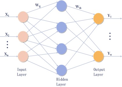
The input signals (, , ) are fed into the input layer and then through the weights and biases () to the hidden layer. The data are then processed in the hidden layer and transmitted to the output layer, where they undergo a nonlinear transformation via the activation function.
The output layer performs a weighted summation and applies the activation function to produce the network’s final output, which is known as the forward propagation of the signal [26], as expressed by Eq. (1):
where, indicates output result; denotes weight from the neuron of the input layer to the neuron of the hidden layer; is the input value; is the bias term of the neuron of the hidden layer.
Secondly, error backpropagation utilizes gradient descent to calculate the deviation between output and real values, which is subsequently propagated backward to adjust the network weights, often evaluated using mean square error (MSE):
where, is the number of sample; is the true value; is the predicted value; is the square of the difference between the true value and the predicted value.
2.2. Mean impact value (MIV)
Determining the input variables is difficult in the practical use of neural network models. Including superfluous or trivial variables in the network input may extend the training period and reduce the model’s accuracy. Thus, the identification of suitable criteria is imperative. Commonly utilized methods for variable selection include principal component analysis, factor analysis, and the mean impact method. Table 1 presents a comparative analysis of their performance.
Table 1Difference of dimensionality reduction methods
Influencing factors | Linear/non-linear | Accuracy | |
PCA | First Principal | Linear | Good |
FA | Specified Factor | Linear | Average |
MIV | Almost no effect | Nonlinear | Better |
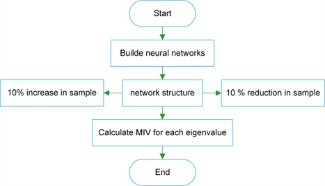
The accuracy and comprehensiveness of the initial data in the MIV algorithm might significantly impact the results, hence requiring data pretreatment [27]. The MIV sign indicates the direction of the independent variable concerning the output variable, while the absolute value represents the magnitude of the effect. Fig. 2 depicts the flowchart of the MIV algorithm, outlining the specific phases as follows [28]:
Step 1: In the neural Network architecture, decrease and increase the training samples by 10 % to create new training samples.
Step 2: The two novel training samples are then simulated utilizing the constructed Network, yielding two simulation outputs. The disparity between these two simulation outcomes is computed, reflecting the variation in impact (Impact Value, IV).
Step 3: The mean of the IV values is computed to derive the MIV (Mean Impact Value) of the Network output.
Step 4: The preceding procedures are reiterated for each independent variable to compute its MIV. The variables are ultimately sorted according to the absolute values of their MIVs, facilitating the assessment of each input feature's impact on the Network’s output.
2.3. Crested porcupine optimizer (CPO)
The crested porcupine optimizer is an innovative optimization method introduced by Abdel-Basset et al., inspired by the four protective behaviors of CP: visual perception, acoustic defense, olfactory recognition, and physical attack [29]. By replicating four behaviors, CPO inherently equilibrates global exploration and local exploitation, hence mitigating the risk of becoming ensnared in local optima. Moreover, in contrast to conventional optimization methods, CPO enhances convergence speed while ensuring the creation of high-quality solutions for intricate multimodal or high-dimensional problems by implementing a periodic population reduction mechanism.
Fig. 2Flowchart of the MIV Algorithm
2.3.1. Initialization phase
In this phase, the CPO operates similarly to other population-based metaheuristic algorithms. CPO begins by randomly initializing a set of candidate solutions, with the initialization formula given by:
where, is the alternative scheme in the solution space, and are the maximums and minimums in space scope, respectively, and is stochastic number from 0 to 1.
2.3.2. Cyclic population reduction
In this phase, the algorithm simulates only the defensive mechanisms activated by threatened crested porcupines. This phase occurs when the population size decreases to a certain threshold, after which the algorithm increases the population size to enhance diversity and accelerate convergence, continuing this process until the maximum number of epochs is reached. The mathematical formula is:
where, is a parameter of the frequency of circulation, is the circulation frequency evaluation, is upper limit, is remainder, is the newly population and is the min number of newly population.
2.3.3. Exploration phase
(1) First and second defense strategies. The CPO algorithm explores the solution by simulating the first two defense mechanisms of the crested porcupine. This phase can be considered a global search in the algorithm, aimed at discovering potentially optimal regions within the solution space. The equation for visual perception is Eq. (5), and the equation for acoustic defense is Eq. (6):
where, is the optimal solution of , predator at the moment position is indicated by , is the stochastic number of normal distribution, and are random values in the interval [0, 1]. and are two stochastic number from .
(2) Third and fourth defense strategies. The CPO algorithm refines the identified optimal region by simulating the last two defense mechanisms of the crown porcupine. This phase can be seen as a local search in the algorithm, aiming to find a more precise solution within the identified region. The equation for olfactory recognition is Eq. (7), and the equation for physical attack defense is Eq. (8):
where, is stochastic number from . is the parameter of the control search route. and are random values in the interval . is the olfactory diffusion factor. is the convergence speed factor, and represents predator for CP strength.
To more intuitively demonstrate the implementation steps of CPO, the pseudocode of CPO is shown in Table 2.
The defense mechanism integrated within the CPO algorithm inherently mitigates the shortcomings of BPNN. The initial and secondary defense mechanisms prioritize global exploration, thus reducing the propensity of BPNN to converge on local minima. Simultaneously, the third and fourth defense mechanisms promote regional development, expediting the convergence to the best solution by identifying prospective areas. The cyclic population reduction process preserves diversity while balancing exploration and exploitation, thus diminishing the susceptibility of BPNN to initial weight selection.
3. Intelligent diagnostic framework for MCB-Net
This study employs CPO to optimize the essential hyperparameters of BPNN adaptively. The fundamental parameters of CPO are established as follows: the number of search people is 8, the maximum number of epochs is 20, and the search boundary is first defined as the interval [−2, 2], which is then increased in accordance with the optimization dimension. The search space of BPNN is set as the number of hidden layer neurons [5, 19], learning rate {0.0001, 0.001, 0.01}, and maximum number of epochs [100, 500]. The range is primarily derived from that utilized in prior studies. An excessively small network size or insufficient training epochs may result in underfitting, whereas an excessively large configuration may substantially elevate computing demands and heighten the danger of overfitting. The objective of optimization is to enhance the classification accuracy of the test set to improve the model’s generalization capability and predictive precision while maintaining convergence efficiency.
Table 3 presents the mean square error (MSE) outcomes associated with varying quantities of hidden layer nodes. The table indicates that the MSE of the network model attains its minimum when the number of hidden layer nodes is 7, thereby establishing 7 nodes as the ideal configuration for the hidden layer. The optimization results for the remaining BPNN hyperparameters are as follows: the maximum number of epochs is 200, and the learning rate is 0.0001. Regarding the Network structure, the number of nodes in the input and output layers is 4 and 10, respectively. The hidden layers use the Tansig activation function, the output layer uses the Purelin activation function, and the training function is Trainlm. In addition, the training and test set sizes are 756 and 324 respectively, the target accuracy is set to 10−6, and the number of failures allowed is 6.
Table 2CPO algorithm pseudocode
Algorithm: Crested Porcupine Optimizer (CPO) Input: Population size Maximum epochs Search space dimension Upper and lower bounds for each dimension Fitness function Output: Best solution Procedure: 1: Initialize population randomly within 2: Evaluate fitness for each candidate 3: Set the best solution 4: For to do 5: For each in population do a) Visual perception: b) Acoustic defense: c) Olfactory recognition: d) Physical attack: where are random numbers in (0,1), and are random individuals from population 6: Apply boundary control to within 7: Evaluate fitness 8: If < , then 9: End 10: Update best solution 11: If cyclic population reduction condition is satisfied: Reduce population by removing worst individuals 12: End Return: |
Table 3Number of nodes in the hidden layer
Number of hidden layer nodes | Training set MSE | Number of hidden layer nodes | Training set MSE |
5 | 0.039342 | 8 | 0.019172 |
6 | 0.030574 | 9 | 0.018585 |
7 | 0.017678 | 10 | 0.018927 |
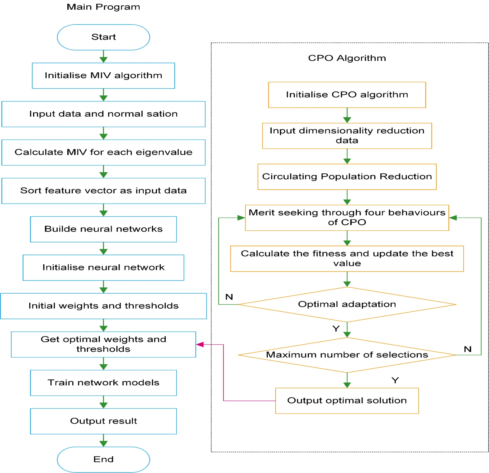
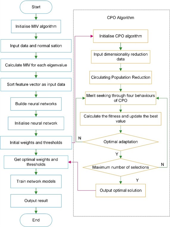
Fig. 3 illustrates the flowchart of the MCB-Net algorithm, with the specific steps for model construction detailed as follows:
Step 1: Enter the bearing data and standardize the data.
Step 2: Organize the feature indicators via the MIV method.
Step 3: Enter the organized feature indicators into the CPO algorithm and BPNN.
Step 4: Initiate the CPO algorithm and neural Network.
Step 5: Assess the population's present fitness utilizing the four defense mechanisms of the CPO algorithm and modify the answer accordingly.
Step 6: Verify if the algorithm has attained optimal fitness. By the fulfillment of prerequisites, proceed to Step 7 and assess whether to iterate towards the maximum. If not, revert to Step 5 to revise the four defensive behaviors of the non-communicating algorithm.
Step 7: Verify if the method has fulfilled the maximum epochs criteria. If satisfied, ascertain the optimal outcome and revise the output accordingly with the best answer. Should the condition remain unfulfilled, revert to step 5 to revise the four defensive behaviors of the non-communicating algorithm.
Step 8: After the CPO algorithm identifies the optimal hyperparameters, train the BPNN and conduct the fault diagnosis.
Fig. 3Flowchart of MCB-Net algorithm
4. Experimental verification
To validate MCB-Net, comparison experiments will be executed against the SVM, Simple CNN (S-CNN), MIV-HO-BP, and MIV-LEA-BP. The efficacy of these approaches will be evaluated based on error, volatility and accuracy. All methodologies will be trained and evaluated utilizing the features extracted in this investigation. All methodologies will be trained and evaluated utilizing the features extracted in this investigation.
The random initialization of neural network parameters in each training session may influence the final output outcomes. To precisely demonstrate the distinction between the optimization model, twenty experimental iterations were done, and the models were assessed utilizing the Mean Squared Error (MSE), Mean Absolute Error (MAE), and Cross-Entropy Loss metrics. The equations for these metrics are presented:
where, is the number of samples; is the true value; is the predicted value; and are the difference and absolute value between the true value and the predicted value. The experimental results show that the MCB-Net algorithm has great advantages of time and accuracy in the paper.
4.1. Feature selection
Table 4 presents the initial nine distinctive indications of bearing faults identified in this study. Indicators 1-4 delineate the statistical properties of the data, whilst the subsequent indicators concentrate on temporal features. The indicators not only signify the extent of bearing failure but may also be integrated with machine learning and fault diagnosis algorithms for categorization, prediction, and fault identification.
Table 4Indicators of bearing failure characteristics
Number | Feature | Number | Feature |
1 | Mean | 6 | Crest factor |
2 | Variance | 7 | Pulse factor |
3 | Peak | 8 | Shape factor |
4 | Kurtosis | 9 | Margin factor |
5 | RMS | – | – |
Fig. 4Characterization indicator importance
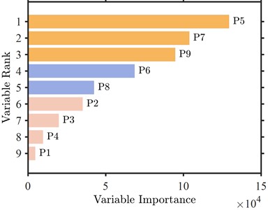
Fig. 4 illustrates the outcomes of the MIV algorithm. In conjunction with Table 4, which present the outcomes of the MIV algorithm, shows the practical value, impact factor, and margin factor to be the three distinctive indicators with the most significant influence on the diagnostic outcomes. The practical value directly indicates the operational condition of the bearing, but the impact factor and margin factor are essential for identifying bearing failure due to impact vibration and assessing the remaining lifespan and severity of failure. Conversely, metrics such as mean, roughness, variability, and peak primarily represent mathematical trends and fail to indicate the bearing condition distinctly. This research identifies the three most influential feature indicators as input variables to enhance the diagnostic model’s accuracy and interpretability while maintaining the features’ validity.
4.2. Case 1
To validate the application of the proposed algorithmic model in real industrial fault diagnosis, this paper first uses the Case Western Reserve University (CWRU) bearing dataset [30]. The CWRU data acquisition setup is shown in Fig. 5. The test bench consists of a variable power motor, a torque transducer, and a power tester, with control electronics. The drive-side bearings are SKF 6205, used for failure tests at 7, 14, and 21 mil diameters at sampling frequencies of 12 kHz and 48 kHz. The fan-side bearings are NTN-equivalent bearings, used for failure tests at 28 mil and 40 mil diameters, with a sampling frequency of 12 kHz.
The data types selected in this study include four conditions: healthy, outer ring failure, inner ring failure, and rolling body failure. Data was collected at diameters of 0.007, 0.014, and 0.021 inches, with a rotational speed of 1797 RPM. The specific data models are shown in Table 5.
Table 5Data types (CWRU)
Type | Diameter (mils) | Diameter (mils) | Diameter (mils) |
Health | – | 1797 | 0 |
Rolling body failure | 7, 14, 21 | 1797 | 0 |
Inner ring failure | 7, 14, 21 | 1797 | 0 |
Outer ring failure | 7, 14, 21 | 1797 | 0 |
Fig. 5CWRU bearing experimental setup
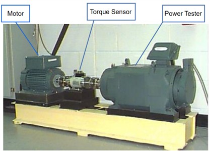
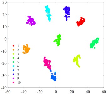
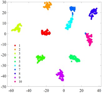
Fig. 6t-SNE visualization
a) S-CNN
b) MIV-LEA-BP
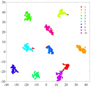
c) SVM
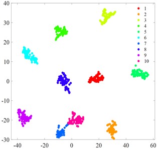
d) MIV-HO-BP
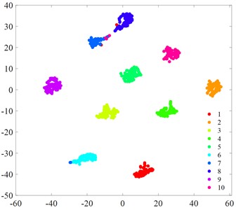
e) MIV-PSO-BP
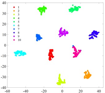
f) MIV-GA-BP
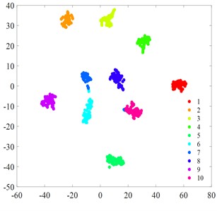
g) MCB-Net
4.2.1. t-SNE visualization
Fig. 6 displays the t-SNE visualization of each algorithmic model. A comparison of the t-SNE plots reveals that the MCB-Net model (Fig. 6(g)) exhibits superior clustering results compared to other models. Specifically, the t-SNE plot of MCB-Net shows clearer category separation and less overlap, which indicates that the model has higher accuracy and efficiency in feature extraction and classification. In addition, the MCB-Net model is able to handle complex nonlinear relationships more efficiently by optimizing the weights and thresholds of the BP neural Network, which improves the prediction accuracy of the model. As shown in the t-SNE plot, data points of different categories form more dispersed and independent clusters in the low-dimensional space.
4.2.2. Accuracy analysis
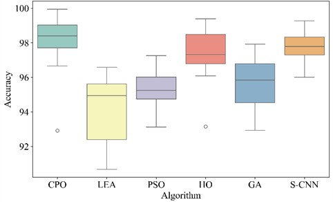
Table 6 shows the accuracy and standard deviation of different methods. Fig. 7 plots the accuracy box plot of different methods under 20 times. As shown in Table 6, MCB-Net achieved an average accuracy of 98.20 %, the highest among all algorithms. The result was 3.95 % higher than the worst-performing LEA and 0.40 % higher than the best-performing S-CNN. Fig. 7 also shows that MCB-Net has the highest accuracy on the vertical axis, with the accuracy of the intermediate data concentrated in the high range. Compared with other algorithms, MIV-LEA-BP has the lowest box position and large fluctuations. The boxes of PSO and GA are also much lower than MCB-Net. Although HO and S-CNN have high performance, the accuracy of the middle segment data of MCB-Net is more concentrated. In addition, the standard deviation of MCB-Net is 1.52 %, second only to S-CNN’s 0.74 % among all models, but its 95 % confidence interval is [97.49, 98.91], which almost covers the upper limit of all other algorithms. The results demonstrate that even with fluctuations, the overall performance of MCB-Net remains significantly higher than that of most algorithms.
Table 6Comparison of various methods (CWRU)
Accuracy | SD | |
MCB-Net | 98.2 % | 1.52 % |
MIV-LEA-BP | 94.25 % | 1.81 % |
MIV-PSO-BP | 95.3 % | 1.21 % |
MIV-HO-BP | 97.35 % | 1.42 % |
MIV-GA-BP | 95.68 % | 1.32 % |
SVM | 96.2 % | 0 |
S-CNN | 97.8 % | 0.74 % |
Fig. 7Box plots of different methods
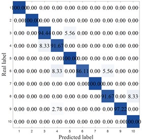
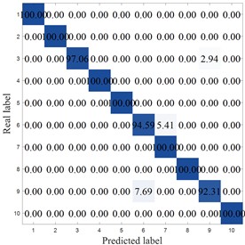
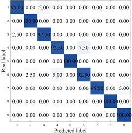
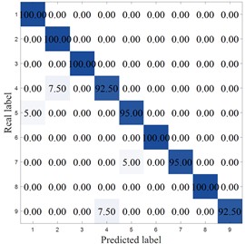
To more clearly demonstrate the results of each method, Fig. 8 shows the confusion matrix of the corresponding model. MCB-Net shows significantly better classification performance than other methods. S-CNN misclassified categories 4, 7, 9, and 10, particularly category 10, where 8.33 % were misclassified as category 6. The SVM correctly classified category 6 only 86.11 %, with a high percentage of misclassifications into category 8 (8.33 %). Misclassifications were also prominent in categories 7, 8, and 9, resulting in the worst overall performance. For example, the optimized algorithm MIV-LEA-BP misclassified 13.89 % of class 3 into class 9, 5.56 % of class 7 into class 6, and 8.33 % into class 9. In contrast, MCB-Net, excluding classes 3, 4, and 9, had a 100 % accuracy rate for all other classes, significantly higher than other methods. The good performance is mainly due to the precise measurement of feature importance by MIV, combined with the efficient optimization of BP neural network parameters by the CPO optimization strategy, which enables the model to more accurately capture the discriminative features of samples, thereby significantly improving the classification accuracy of samples in each category and effectively reducing the degree of confusion between categories.
Fig. 8Accuracy analysis
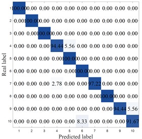
a) S-CNN
b) MIV-LEA-BP
c) SVM
d) MIV-HO-BP
e) MIV-GA-BP
f) MIV-PSO-BP
g) MCB-Net
4.2.3. Error analysis
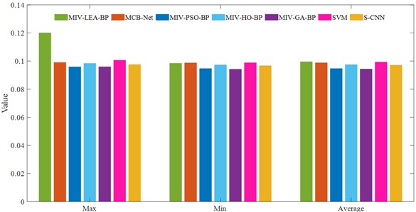
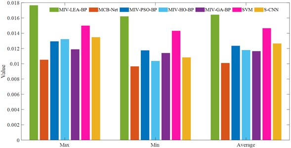
This research quantitatively evaluates the merits and demerits of the four algorithms by conducting 20 epochs for each and use MAE and MSE as comparative assessment measures. Table 7 and 8 present the MAE and MSE for each approach. Excluding MCB-Net, the MAE indicator reveals that the average error values of the remaining methods are clustered between 0.037 and 0.043. Notably, MIV-PSO-BP exhibits the lowest average error at 0.037432; however, the discrepancy between the maximum and minimum values is considerable, suggesting that its overall performance stability is moderate. The average MAE of MCB-Net is 0.045083, marginally above that of certain approaches; however, the disparity between its highest and minimum values is merely 0.001884, indicating substantial stability and consistency. The fluctuation ranges of other approaches, specifically MIV-HO-BP and S-CNN, are 0.002398 and 0.000472, respectively, signifying a degree of uncertainty in both under varying operating conditions.
Table 7MAE comparison of four algorithms (CWUR)
Max value | Min value | Average value | |
MIV-LEA-BP | 0.040012 | 0.039854 | 0.039972 |
MCB-Net | 0.046399 | 0.044515 | 0.045083 |
MIV-PSO-BP | 0.042233 | 0.036244 | 0.037432 |
MIV-HO-BP | 0.044272 | 0.042982 | 0.043163 |
MIV-GA-BP | 0.041637 | 0.038627 | 0.040132 |
SVM | 0.043348 | 0.042622 | 0.043118 |
S-CNN | 0.042641 | 0.042169 | 0.042547 |
Table 8MSE comparison of four algorithms (CWUR)
Max value | Min value | Average value | |
MIV-LEA-BP | 0.015375 | 0.014287 | 0.014559 |
MCB-Net | 0.010019 | 0.009628 | 0.009752 |
MIV-PSO-BP | 0.011886 | 0.011607 | 0.011632 |
MIV-HO-BP | 0.012646 | 0.010248 | 0.011427 |
MIV-GA-BP | 0.011807 | 0.011377 | 0.011570 |
SVM | 0.012957 | 0.010365 | 0.011430 |
S-CNN | 0.013502 | 0.010801 | 0.012762 |
In terms of MSE indicators, the advantage of MCB-Net is more obvious, with an average MSE of only 0.009752, which is significantly lower than other methods. Specifically, MCB-Net is 33 % higher than MIV-LEA-BP and 15 % higher than MIV-PSO-BP and MIV-GA-BP. In addition, the gap between the maximum and minimum values of MCB-Net is only 0.000391, further demonstrating that it can maintain highly consistent prediction performance. To more clearly demonstrate the differences between the methods, Fig. 9 plots the MAE and MSE comparisons for each method. The figure clearly shows that MCB-Net has the most significant overall advantage in MSE. In contrast, the other algorithms have higher mean errors or larger fluctuations in MSE, indicating greater instability in their prediction results.
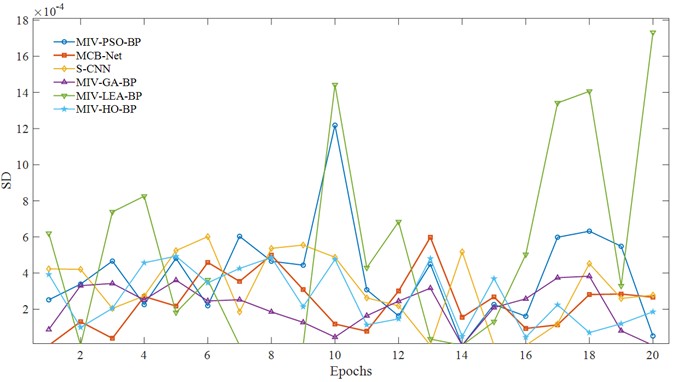
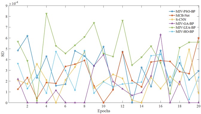
4.2.4. Volatility analysis
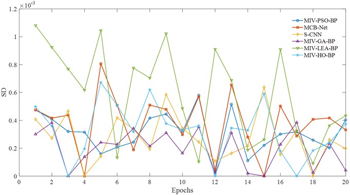
Algorithm volatility is commonly used to evaluate the stability and predictability of its performance. This study conducted 20 independent epochs for each algorithm to analyze its convergence behavior. Fig. 10 illustrates the volatility of each algorithm during epochs. The horizontal axis represents the number of epochs, while the vertical axis shows the SD of the convergence curve, reflecting the degree of convergence fluctuation within a single run. Higher values on the vertical axis indicate lower convergence stability during that epochs. It should be noted that since the performance of SVM is extremely stable, volatility is not plotted. From the figure, we can see that the MCB-Net curve shows much better stability than other algorithms during the 20 epochs. Specifically, MIV-PSO-BP and MIV-LEA-BP experience large fluctuations during epochs, and the S-CNN model exhibits large local interference. However, the overall fluctuation amplitude of the CPO curve is gentle and regular, indicating that when MCB-Net adjusts the BP neural network parameters through the CPO optimization strategy, combined with MIV's precise measurement of feature importance, the model can more stably approach the optimal solution during training epochs.
Fig. 9MAE and MSE comparison of four algorithms (CWUR)
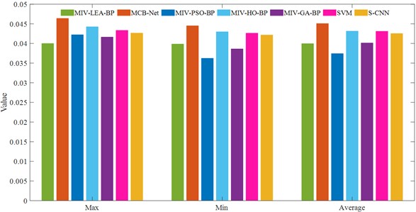
a) MAE
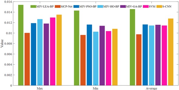
b) MSE
Fig. 10Volatility across algorithms
4.3. Case 2
In order to verify the generalization ability and robustness of the algorithm model proposed in this paper, the bearing data of Society for Machinery Failure Prevention Technology (MFPT) [31] in the United States are selected. The data set is also a public data set. Compared with CWUR, it only records inner ring faults, outer ring faults and normal states. Table 9 is selected data types of MFPT.
Table 9Selected data types (MFPT)
Type | Roller diameter | Load | Sampling frequency |
Health | 0.235 | 270 | 48828 |
Outer ring fault | 0.235 | 50, 100, 270 (3) | 48828 |
Inner ring fault | 0.235 | 50, 150, 300 | 48828 |
4.3.1. Accuracy analysis
Table 10 and Fig. 11 show the performance of different methods. The accuracy of MCB-Net reached 97.26 %, the highest among all methods, an improvement of 1.06 % compared to SVM and 1 % compared to S-CNN’s 96.93 %. Compared with other optimization algorithms, the accuracy of BPNN optimized by CPO is improved by 2.03 %. Further combining the SD, we can see that MCB-Net's SD is only 1.05%, indicating that its results are less volatile across multiple experiments and exhibit greater stability. Although S-CNN’s SD is 0.83 %, showing better stability, its accuracy is still lower than MCB-Net, indicating that CPO achieves a better balance between stability and accuracy. The box plot results further show that the distribution range of MCB-Net is more compact and its overall position is higher, which means that it cannot only remain stable in different experiments but also achieve better performance.
Table 10Comparison of various methods (MFTP)
Accuracy | SD | |
MCB-Net | 97.26 % | 1.05 % |
MIV-LEA-BP | 94.81 % | 1.68 % |
MIV-PSO-BP | 95.23 % | 1.43 % |
MIV-HO-BP | 96.70 % | 1.31 % |
MIV-GA-BP | 95.08 % | 1.48 % |
SVM | 96.2 % | 0 |
S-CNN | 96.93 % | 0.83 % |
Fig. 11Box plot of different methods (MFTP)
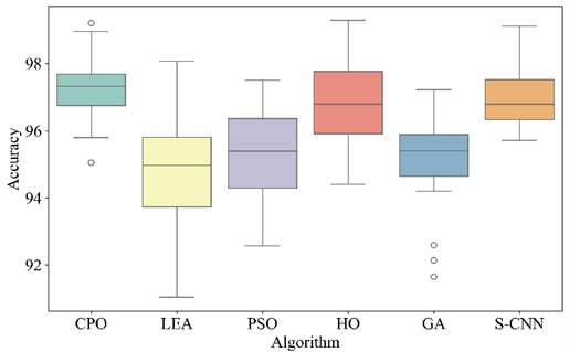
Fig. 12Accuracy analysis
a) S-CNN
b) MIV-LEA-BP
c) SVM
d) MIV-HO-BP
e) MIV-GA-BP
f) MIV-PSO-BP
g) MCB-Net
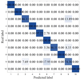
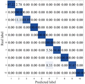
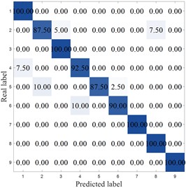
Fig. 12 shows the confusion matrix of different methods. As can be seen from the figure, except for MCB-Net and MIV-PSO-BP, the other algorithms all made misclassifications in category 1. The LEA-optimized model had the largest classification errors, with significant misclassifications in categories 1, 6, 7, 8, and 9. The SVM performed second worst, primarily in categories 4, 7, and 8. Meanwhile, the MCB-Net achieved accuracy rates above 95 % for all categories except categories 2 and 9. Other algorithms, such as S-CNN and SVM, exhibit relatively high values in some off-diagonal locations. Judging from the confusion matrix, the MCB-Net algorithm demonstrates superior classification performance, thanks to CPO's fine-tuning of model parameters during the optimization process, which better captures data features and thus excels in multi-class classification tasks.
4.3.2. Error analysis
In this dataset, the same 20 experimental epochs were conducted, and the selection of evaluation index parameters aligned with the CWUR dataset. The results for MAE and MSE are presented in Table 11 and 12, as well as Fig. 13. As can be seen from the table, the MCB-Net algorithm shows both balance and superiority. The maximum MAE is 0.099026, which is significantly lower than 0.120079 of MIV-LEA-BP and 0.100611 of SVM. It effectively avoids large deviations in the prediction process, thereby reducing the adverse effects of extreme errors on the overall performance. Although the minimum value is 0.098726, which is slightly higher than some optimization algorithms, the difference between the maximum and minimum values is only about 0.0003, highlighting its robustness in terms of control errors. The MSE indicator shows that compared with other methods, the average MSE is only slightly higher than S-CNN's 0.037496, and the overall performance is superior. In addition, the difference between the maximum and minimum MSE values is only about 0.0010, which is much smaller than 0.0037 of MIV-LEA-BP and 0.0023 of MIV-HO-BP. The visualization in Fig. 13 more directly demonstrates the performance of MCB-Net. With the exception of LEA, which has a significantly higher MAE, the other algorithms are largely comparable. A comparison of MSE reveals that MCB-Net achieves the best performance, further validating its ability to achieve high accuracy and stability in complex prediction tasks.
Table 11MAE comparison of four algorithms (MFPT)
Max value | Min value | Average value | |
MIV-LEA-BP | 0.120079 | 0.098434 | 0.099516 |
MCB-Net | 0.099026 | 0.098726 | 0.098756 |
MIV-PSO-BP | 0.095914 | 0.094645 | 0.094676 |
MIV-HO-BP | 0.098378 | 0.097305 | 0.097498 |
MIV-GA-BP | 0.095932 | 0.094169 | 0.094307 |
SVM | 0.100611 | 0.098835 | 0.099279 |
S-CNN | 0.097552 | 0.096730 | 0.097141 |
Table 12MSE comparison of four algorithms (MFPT)
Max value | Min value | Average value | |
MIV-LEA-BP | 0.041940 | 0.038204 | 0.038391 |
MCB-Net | 0.037735 | 0.036714 | 0.036816 |
MIV-PSO-BP | 0.038518 | 0.037426 | 0.037851 |
MIV-HO-BP | 0.039606 | 0.037270 | 0.037854 |
MIV-GA-BP | 0.038047 | 0.037943 | 0.037985 |
SVM | 0.039956 | 0.038175 | 0.038898 |
S-CNN | 0.037881 | 0.037112 | 0.037496 |
4.3.3. Volatility analysis
Fig. 14 shows the SD of the convergence curves of each algorithm after 20 epochs. Overall, the MCB-Net algorithm has a very small standard deviation fluctuation during the entire iteration process, showing high stability. In contrast, the standard deviation curve of the PSO algorithm fluctuates greatly from the 10th to the 15th iteration, indicating that its optimization effect is unstable at this stage.
Fig. 13MAE and MSE comparison of four algorithms (MFPT)
a) MAE
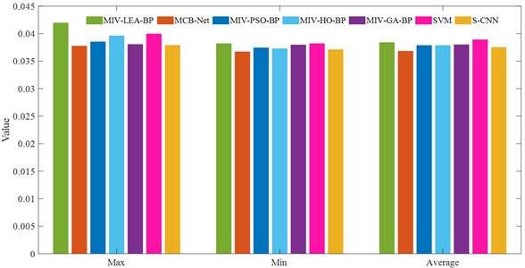
b) MSE
Fig. 14Volatility of the MFPT bearing dataset
The LEA algorithm also experienced similar dramatic fluctuations between the 5th and 10th epochs, indicating that its optimization process at this stage was greatly disturbed. Although the S-CNN and HO algorithms showed a certain downward trend in the middle and late stages, the overall fluctuation range was still higher than that of the MCB-Net algorithm, and the convergence speed was relatively slow, failing to effectively suppress the uncertainty in the training process. For example, after the 15th iteration, the HO standard deviation curve shows a significant rebound. MCB-Net effectively reduces the randomness and uncertainty in the optimization process through optimized control strategies and improved update mechanisms, enabling the algorithm to converge more smoothly to the optimal solution.
4.4. Case 3
In this section, the data used in the experiment were provided by Southeast University, and the faults such as Inner ring fault, Outer ring fault, and Ball fault were recorded [32]. Fig. 15 shows the test bench, which consists of a motor controller, Planetary Gear box, and other components. Records data for 0 V load and 2 V at 20 Hz and 30 Hz speeds, respectively. Table 13 shows the data used in this experiment.
Fig. 15SEU test bench
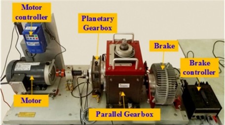
Table 13Experimental data
Type | Speeds (Hz) | Load (V) |
Health | 20 | 0 |
Inner ring fault | 20 | 0 |
Outer ring fault | 20 | 2 |
Ball fault | 20 | 0 |
Outer and inner ring fault | 20 | 2 |
4.4.1. Accuracy analysis
Table 14 shows the comparative experimental results of various methods on the SEU dataset. From the experimental results of the SEU dataset presented in the table, the MCB-Net method achieved the highest accuracy of 97.78 %, with a standard deviation of 0.98 %, showing good stability. Although MIV-HO-BP is close in accuracy, reaching 96.82 %, its standard deviation is 1.10 %, indicating that MCB-Net has more consistent classification performance while maintaining high accuracy.
Table 14Comparison of various methods (SEU)
Accuracy | SD | |
MCB-Net | 97.78 % | 0.98 % |
MIV-LEA-BP | 95.19 % | 1.05 % |
MIV-PSO-BP | 95.83 % | 1.22 % |
MIV-HO-BP | 96.82 % | 1.10 % |
MIV-GA-BP | 95.64 % | 1.16 % |
SVM | 96.30 % | 0 |
S-CNN | 97.32 % | 0.78 % |
Fig. 16Box plot of different methods (SEU)
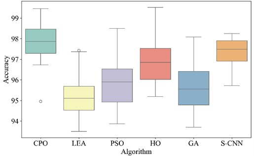
Fig. 17Accuracy analysis
a) S-CNN
b) MIV-LEA-BP

c) SVM
d) MIV-HO-BP
e) MIV-GA-BP
f) MIV-PSO-BP
g) MCB-Net
Fig. 16 is a box plot of each method under the SEU dataset. Fig. 16 shows that the overall distribution of MCB-Net is relatively concentrated, and the median position is relatively high. However, it must be pointed out that MCB-Net has only outliers compared with other algorithms, indicating that there is still room for improvement in stability under extreme conditions.
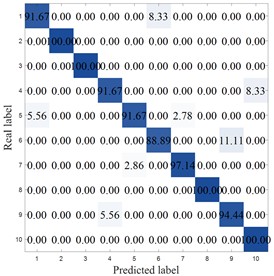
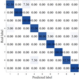
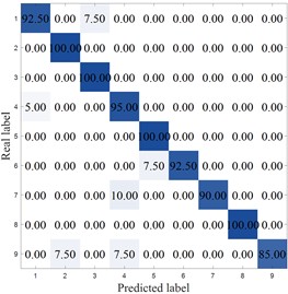
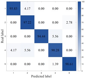
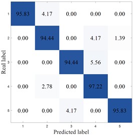
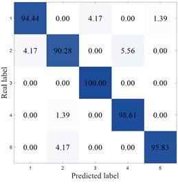
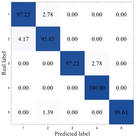
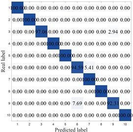
Fig. 17 plots the confusion matrix for the SEU dataset. From the confusion matrix, MCB-Net performs outstandingly in classification performance, and the prediction accuracy of each category is at a high level. Compared with other models, MCB-Net's overall accuracy and single category accuracy are better than most comparison models. For example, the 100 % accuracy for category 4 and 98.61 % for category 5 are far higher than the performance of some models in this category. At the same time, the accuracy of other categories such as categories 1, 2, and 3 also remains at a high level, and the misclassification rate is extremely low (for example, only 2.78 % of category 1 is misclassified as category 2, and only 2.78 % of category 3 is misclassified as category 4). This shows that MCB-Net has stronger discrimination between categories, better overall classification stability and accuracy, and can complete multi-category classification tasks more accurately than other models.
4.4.2. Error analysis
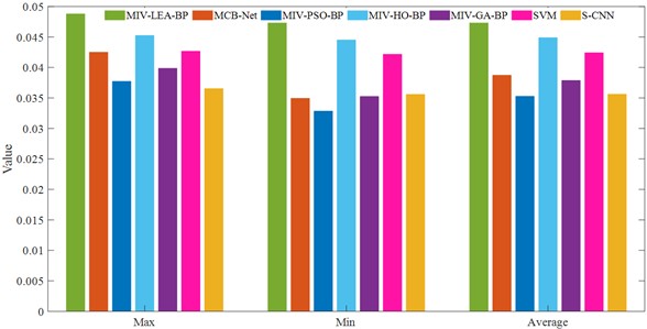
Table 15 and Table 16 show the comparison of error indicators under the SEU dataset. The MCB-Net algorithm demonstrated excellent performance. As shown in Table 15, MCB-Net also outperformed most of the comparison algorithms, with its average MAE only about 0.01 lower than the best-performing MIV-PSO-BP (0.037723) and S-CNN (0.036540) models. As can be seen from Table 16, the average value of MCB-Net is significantly lower than that of other comparison methods. Compared with MIV-LEA-BP, its MSE is reduced by 38.6 %, which fully demonstrates its core advantage in accuracy. At the same time, the maximum and minimum MSE values of MCB-Net are maintained at a low level, indicating that the algorithm has strong robustness and can effectively avoid extreme errors. Overall, MCB-Net has an absolute advantage in the MSE indicator, which more severely penalizes large errors, confirming its comprehensive superiority in improving the overall prediction accuracy and stability of the model.
Table 15MAE comparison of four algorithms (SEU)
Max value | Min value | Average value | |
MIV-LEA-BP | 0.048782 | 0.047714 | 0.047479 |
MCB-Net | 0.042512 | 0.034950 | 0.038731 |
MIV-PSO-BP | 0.037723 | 0.032839 | 0.035281 |
MIV-HO-BP | 0.045250 | 0.044515 | 0.044883 |
MIV-GA-BP | 0.039872 | 0.035250 | 0.037863 |
SVM | 0.042670 | 0.042169 | 0.042420 |
S-CNN | 0.036540 | 0.035586 | 0.035609 |
Table 16MSE comparison of four algorithms (SEU)
Max value | Min value | Average value | |
MIV-LEA-BP | 0.017643 | 0.016198 | 0.016421 |
MCB-Net | 0.010512 | 0.009645 | 0.010079 |
MIV-PSO-BP | 0.012924 | 0.011745 | 0.012335 |
MIV-HO-BP | 0.013213 | 0.010350 | 0.011782 |
MIV-GA-BP | 0.011875 | 0.011391 | 0.011633 |
SVM | 0.014987 | 0.014300 | 0.014644 |
S-CNN | 0.013472 | 0.010820 | 0.012646 |
Fig. 18 provides an intuitive display of MAE and MSE. The MCB-Net algorithm outperforms all other comparison models in terms of MSE. Its maximum, minimum, and average MSE values are all at the lowest, significantly lower than those of models like MIV-LEA-BP and SVM. In MAE, the average performance of MCB-Net is close to that of the optimal model, and the maximum value of MAE is significantly lower than that of BPNN optimized by other algorithms, showing a more stable error upper limit control ability.
Fig. 18MAE and MSE comparison of four algorithms (SEU)
a) MAE
b) MSE
4.4.3. Volatility analysis
Fig. 19 shows the SD of the convergence curve under the SEU dataset. As can be seen from the figure, the convergence error of MCB-Net shows a lower fluctuation amplitude and a more stable downward trend overall. In the first five cycles, the error decreased rapidly and remained at a low level, while the LEA model had obvious peak fluctuations. In the 5th to 15th cycles, although there are some fluctuations, the error fluctuation of MCB-Net is significantly smaller than that of PSO, S-CNN and other algorithms. Later in the cycle, the error continues to decrease steadily. This low volatility and high stability stems from MIV's effective screening of input information and CPO’s precise control of the optimization process. The synergistic effect of the two enables the algorithm to avoid local optimal traps during training, while improving convergence efficiency and robustness. Compared with other algorithms, MCB-Net not only achieves a faster convergence speed within 20 cycles, but more importantly, its error fluctuation is effectively suppressed, reflecting the algorithm's stronger anti-interference ability and generalization performance in complex optimization tasks.
Fig. 19Volatility across algorithms
4.5. Convergence performance and ablation experiment
4.5.1. Convergence performance test
To comprehensively evaluate the convergence performance of the CPO algorithm, this study selected commonly used multimodal benchmark test functions for experiments to verify its capabilities in global search and local development. All test functions solved in this paper have a dimension of 10, and the population size and number of epochs are 30 and 100, respectively. Multimodal functions contain multiple local extreme points and are often used to test the optimizer’s ability to explore and escape from local optimality.
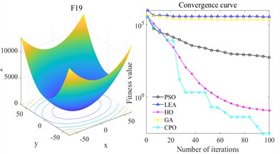
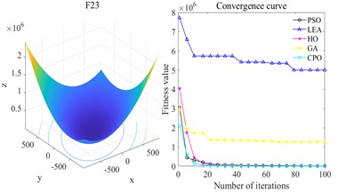
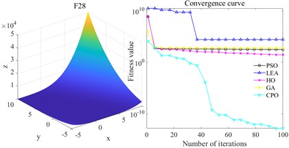
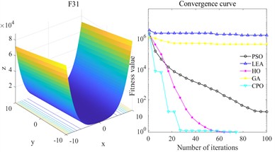
Fig. 20 shows the convergence curves of each algorithm. Overall, the advantages of CPO are particularly significant. Taking F19 as an example, LEA and GA show an overall slow decline during the iteration process, always maintaining a high fitness level, and the final result is significantly inferior to CPO; although PSO and HO can gradually reduce the fitness value, there is a gap in both convergence speed and final accuracy, while CPO can decline rapidly in the initial stage and eventually reach convergence. In terms of convergence speed, CPO’s rate of decline on all functions is significantly greater than that of the other compared algorithms. In F23, although GA and HO have certain optimization trends, their rate of decline is slower than that of CPO, and their final results are much higher than CPO. CPO can converge quickly and reach the optimal value at an early stage. The results of F28 further highlight the differences. Except for CPO, the fitness values of the other optimization algorithms always remain at a high level. From the perspective of convergence accuracy, the final fitness value of CPO always remains at the lowest level and is relatively stable. Specifically, on F31, LEA maintains a high level and hardly converges. GA, PSO, and HO converge significantly slower than CPO.
In summary, CPO has both strong exploration efficiency and local convergence capabilities in the tested multimodal functions, and can obtain better solutions within a limited number of epochs, demonstrating its stability and advantages in complex optimization problems.
Fig. 20Multimodal benchmark function test
a) F19
b) F23
c) F28
d) F31
4.5.2. Ablation experiment
In this subsection, systematic ablation experiments are conducted to verify the synergistic effect of the proposed algorithm in this paper. Due to the comparison of other optimizations in subsection 4.1.3, there are only two groups of experiments: Experiment 1 using only BPNN for diagnosis and Experiment 2 using MIV-BPNN. Each group of experiments is run independently on the CWRU dataset with the same Network structural parameters to eliminate the effect of randomness.
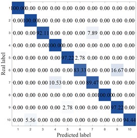
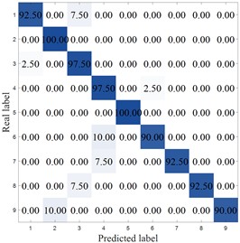
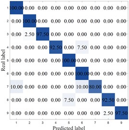
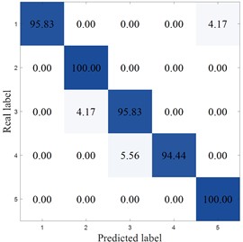
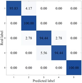
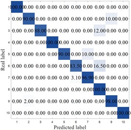
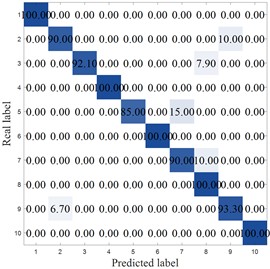
Fig. 21 shows the confusion matrix of Experiment 1 and Experiment 2. As can be seen from the figure, the classification performance of a single BP model fluctuates to a certain extent. For example, the recognition rate for categories 6 and 7 is only 83.5 %, and the generalization ability is limited when processing certain complex patterns. The MIV-BP model improves the accuracy to 95.8 %, mainly due to the MIV algorithm's selection of characteristic indicators, which eliminates the influence of other interfering indicators on the results. The MCB-Net model achieved an even higher accuracy rate of 98.2 %. First, the MIV algorithm precisely selected the features that contributed most to classification, achieving 100 % accuracy for categories 2 and 8 while minimizing interference from other information. Second, the CPO algorithm further optimized network parameters, avoiding local optimal solutions through global search. This significantly increased the model’s recognition rate for complex categories (such as categories 6 and 7) from 83.5 % to 94.59 %, while also achieving enhanced recognition stability across all categories. In comparison, MCB-Net not only inherits the feature selection capability of MIV, but also enhances the robustness and convergence efficiency of the model through the dynamic parameter adjustment mechanism of CPO, and ultimately achieves near-optimal performance in classification tasks.
In addition, combining subsection 4.1.2 with other optimization algorithms, best-performing optimization algorithm, MIV-HO-BP, achieved an accuracy rate of 97.35 %, MIV-LEA-BP is 94.25 %, MIV-PSO-BP is 95.3 %, and BPNN performs the best after optimization with MIV feature selection and post-CPO algorithm. This result not only reflects the necessity of feature selection to reduce redundancy and improve model efficiency but also the advantages of the CPO algorithm.
Fig. 21Experiment 1 and Experiment 2 confusion matrices
a) BP
b) MIV-BP
c) MCB-Net
4.6. Discussion
The fault diagnosis approach presented in this paper, utilizing MIV and CPO-optimized BPNN, demonstrates considerable performance benefits. The ablation experiment depicted in Fig. 21 indicates that the practical value, impact factor, and margin factor identified by MIV substantially influence the performance of the BP neural network. When solely these high-impact characteristics are maintained as input, the model’s diagnostic accuracy improves by 14.73 % relative to the original BP, hence underscoring the efficacy of MIV in feature extraction. MIV not only markedly improves model performance but also mitigates the black box issue of deep models to some degree, rendering the diagnostic procedure more comprehensible. In the parameter optimization phase, CPO exhibited enhanced convergence properties and predictive accuracy relative to conventional optimization algorithms like GA, PSO, and LEA, achieving optimal MSE and MAE metrics performance. Fig. 20 indicates that CPO has superior convergence efficiency compared to other optimization techniques.
This study empirically corroborates the MCB-Net model utilizing three bearing datasets across various operational situations. The findings indicate that the MCB-Net classification accuracy consistently exceeds 97 % with a minimal standard deviation across all three datasets. Demonstrating consistent diagnostic performance across various operational settings and failure modes, MCB-Net showcases significant robustness and generalization abilities. The advantages of MCB-Net differ from GA’s dependence on selection, crossover, and mutation and PSO’s reliance on individual and collective flight experience. CPO attains a dynamic equilibrium between global and local search by emulating the four defensive behaviors of porcupines, and enhances convergence through a cyclic population reduction strategy, thereby effectively mitigating the risk of local optimality and ensuring the model's superior performance across various tasks.
Moreover, the excellence of DL models like CNNs and GCNs in intricate feature extraction is offset by practical implementation challenges stemming from computational constraints at industrial sites. The CPO-BPNN, in conjunction with MIV feature selection, guarantees precise diagnosis and offers interpretable input metrics, rendering the method more appropriate for resource-limited industrial applications while maintaining a balance between performance and efficiency.
5. Conclusions
This study presents MCB-Net, an intelligent diagnostic system for resource-constrained industrial environments. MCB-Net leverages the minimal parameters and low computational demands of BPNN, integrating it with MIV feature selection and CPO optimization skills to get enhanced accuracy. The main conclusions of this paper are as follows:
1) Introduces the MIV method to effectively screen out key features and reduce the input dimension, thereby alleviating the overfitting risk of BPNN in high-dimensional environments while also improving model interpretability and enhancing the transparency of diagnostic results.
2) The introduction of the CPO algorithm significantly improves the shortcomings of traditional BPNN in terms of slow convergence speed and easy falling into local optimality. Compared with optimization methods such as PSO and GA, CPO has stronger global search capabilities and higher convergence efficiency, thereby effectively improving diagnostic accuracy and stability.
3) Experimental results on three different working condition datasets show that MCB-Net outperforms existing methods in diagnostic accuracy, robustness, and stability, verifying its application potential in actual industrial scenarios.
However, this approach still has limitations, such as lack of applicability in high-noise environments, extreme fault types, and multi-bearing systems. Future research will focus on improving noise robustness, extending to multi-source sensor data fusion, and combining transfer learning with federated learning to enhance generalization capabilities under different operating conditions.
References
-
X. Zhang, X. Zhang, W. Liang, and F. He, “Research on rolling bearing fault diagnosis based on parallel depthwise separable ResNet neural network with attention mechanism,” Expert Systems with Applications, Vol. 286, p. 128105, Aug. 2025, https://doi.org/10.1016/j.eswa.2025.128105
-
Z. Chen et al., “Research on bearing fault diagnosis based on improved genetic algorithm and BP neural network,” Scientific Reports, Vol. 14, No. 1, p. 128105, Jul. 2024, https://doi.org/10.1038/s41598-024-66318-0
-
G. Bai et al., “Unsupervised multiple-target domain adaptation for bearing fault diagnosis,” Engineering Applications of Artificial Intelligence, Vol. 154, p. 111063, Aug. 2025, https://doi.org/10.1016/j.engappai.2025.111063
-
B. Zhang, S. Wan, X. Zhao, C. Wang, X. Zhang, and X. Sheng, “Instantaneous rotational frequency estimation and fault diagnosis for rotating machinery based on multi-component short-time Fourier transform,” Measurement, Vol. 253, p. 117565, Sep. 2025, https://doi.org/10.1016/j.measurement.2025.117565
-
Z. Gao, J. Zheng, H. Pan, J. Cheng, and J. Tong, “Translational Gaussian wavelet transform and its application to the fault diagnosis of rolling bearing,” Nonlinear Dynamics, Vol. 113, No. 20, pp. 27483–27499, Jul. 2025, https://doi.org/10.1007/s11071-025-11553-x
-
K. Sun and A. Yin, “Multi-sensor temporal-spatial graph network fusion empirical mode decomposition convolution for machine fault diagnosis,” Information Fusion, Vol. 114, p. 102708, Feb. 2025, https://doi.org/10.1016/j.inffus.2024.102708
-
Q. Zhang and Z. Ju, “Rolling bearing fault diagnosis based on 2D CNN and hybrid kernel fuzzy SVM,” Advanced Theory and Simulations, Vol. 8, No. 6, p. 24007, Feb. 2025, https://doi.org/10.1002/adts.202400793
-
L. Wan, K. Gong, G. Zhang, X. Yuan, C. Li, and X. Deng, “An efficient rolling bearing fault diagnosis method based on spark and improved random forest algorithm,” IEEE Access, Vol. 9, pp. 37866–37882, Jan. 2021, https://doi.org/10.1109/access.2021.3063929
-
Y. Lu and Z. Huang, “A new hybrid model of sparsity empirical wavelet transform and adaptive dynamic least squares support vector machine for fault diagnosis of gear pump,” Advances in Mechanical Engineering, Vol. 12, No. 5, p. 16878, May 2014, https://doi.org/10.1177/1687814020922047
-
A. B. Patil, J. A. Gaikwad, and J. V. Kulkarni, “Bearing fault diagnosis using discrete wavelet transform and artificial neural network,” in 2nd International Conference on Applied and Theoretical Computing and Communication Technology (iCATccT), pp. 399–405, Jan. 2016, https://doi.org/10.1109/icatcct.2016.7912031
-
Z. Wang, Q. Zhang, J. Xiong, M. Xiao, G. Sun, and J. He, “Fault diagnosis of a rolling bearing using wavelet packet denoising and random forests,” IEEE Sensors Journal, Vol. 17, No. 17, pp. 5581–5588, Sep. 2017, https://doi.org/10.1109/jsen.2017.2726011
-
Z. Li, H. Jiang, and Y. Dong, “A convolutional-transformer reinforcement learning agent for rotating machinery fault diagnosis,” Expert Systems with Applications, Vol. 271, p. 126669, May 2025, https://doi.org/10.1016/j.eswa.2025.126669
-
Y. Zhang, S. Zhang, Y. Zhu, and W. Ke, “Cross-domain bearing fault diagnosis using dual-path convolutional neural networks and multi-parallel graph convolutional networks,” ISA Transactions, Vol. 152, pp. 129–142, Sep. 2024, https://doi.org/10.1016/j.isatra.2024.06.009
-
L. Cui, X. Tian, Q. Wei, and Y. Liu, “A self-attention based contrastive learning method for bearing fault diagnosis,” Expert Systems with Applications, Vol. 238, p. 121645, Mar. 2024, https://doi.org/10.1016/j.eswa.2023.121645
-
L. Wen, X. Li, and L. Gao, “A transfer convolutional neural network for fault diagnosis based on ResNet-50,” Neural Computing and Applications, Vol. 32, No. 10, pp. 6111–6124, Feb. 2019, https://doi.org/10.1007/s00521-019-04097-w
-
Y. Du, A. Wang, S. Wang, B. He, and G. Meng, “Fault diagnosis under variable working conditions based on stft and transfer deep residual network,” Shock and Vibration, Vol. 2020, pp. 1–18, May 2020, https://doi.org/10.1155/2020/1274380
-
X. Liu, L. Xia, J. Shi, L. Zhang, L. Bai, and S. Wang, “A fault diagnosis method of rolling bearing based on improved recurrence plot and convolutional neural network,” IEEE Sensors Journal, Vol. 23, No. 10, pp. 10767–10775, May 2023, https://doi.org/10.1109/jsen.2023.3265409
-
N. Zhang, Y. Li, X. Yang, and J. Zhang, “Bearing fault diagnosis based on bp neural network and transfer learning,” in Journal of Physics: Conference Series, Vol. 1881, No. 2, p. 022084, Apr. 2021, https://doi.org/10.1088/1742-6596/1881/2/022084
-
Y. Liu, J. Kang, Y. Bai, and C. Guo, “Research on the health status evaluation method of rolling bearing based on EMD‐GA‐BP,” Quality and Reliability Engineering International, Vol. 39, No. 5, pp. 2069–2080, Apr. 2023, https://doi.org/10.1002/qre.3350
-
S. Chen and S. Zou, “Enhancing bearing fault diagnosis with deep learning model fusion and semantic web technologies,” International Journal on Semantic Web and Information Systems, Vol. 20, No. 1, pp. 1–20, Oct. 2024, https://doi.org/10.4018/ijswis.356392
-
Y. Gao, J. Zhang, Y. Wang, J. Wang, and L. Qin, “Love evolution algorithm: a stimulus-value-role theory-inspired evolutionary algorithm for global optimization,” The Journal of Supercomputing, Vol. 80, No. 9, pp. 12346–12407, Feb. 2024, https://doi.org/10.1007/s11227-024-05905-4
-
M. H. Amiri, N. Mehrabi Hashjin, M. Montazeri, S. Mirjalili, and N. Khodadadi, “Hippopotamus optimization algorithm: a novel nature-inspired optimization algorithm,” Scientific Reports, Vol. 14, No. 1, p. 5032, Feb. 2024, https://doi.org/10.1038/s41598-024-54910-3
-
L. Deng, C. Zhao, X. Yan, Y. Zhang, and R. Qiu, “A novel approach for bearing fault diagnosis in complex environments using PSO-CWT and SA-FPN,” Measurement, Vol. 249, p. 117027, May 2025, https://doi.org/10.1016/j.measurement.2025.117027
-
D. E. Rumelhart, G. E. Hinton, and R. J. Williams, “Learning representations by back-propagating errors,” Nature, Vol. 323, No. 6088, pp. 533–536, Oct. 1986, https://doi.org/10.1038/323533a0
-
J. Li, X. Yao, X. Wang, Q. Yu, and Y. Zhang, “Multiscale local features learning based on BP neural network for rolling bearing intelligent fault diagnosis,” Measurement, Vol. 153, p. 107419, Mar. 2020, https://doi.org/10.1016/j.measurement.2019.107419
-
B. Zhang et al., “A fault diagnosis method for cycloidal hydraulic motors based on improved BP neural network and fusion feature vectors,” Journal of the Brazilian Society of Mechanical Sciences and Engineering, Vol. 47, No. 11, p. 98580, Sep. 2025, https://doi.org/10.1007/s40430-025-05823-3
-
C.-Y. Lee and H.-Y. Ou, “Induction motor multiclass fault diagnosis based on mean impact value and PSO-BPNN,” Symmetry, Vol. 13, No. 1, p. 104, Jan. 2021, https://doi.org/10.3390/sym13010104
-
S. Luo, J. Cheng, and K. Wei, “A fault diagnosis model based on LCD-SVD-ANN-MIV and VPMCD for Rotating Machinery,” Shock and Vibration, Vol. 2016, pp. 1–10, Jan. 2016, https://doi.org/10.1155/2016/5141564
-
M. Abdel-Basset, R. Mohamed, and M. Abouhawwash, “Crested porcupine optimizer: a new nature-inspired metaheuristic,” Knowledge-Based Systems, Vol. 284, p. 111257, Jan. 2024, https://doi.org/10.1016/j.knosys.2023.111257
-
W. A. Smith and R. B. Randall, “Rolling element bearing diagnostics using the Case Western Reserve University data: A benchmark study,” Mechanical Systems and Signal Processing, Vol. 64-65, pp. 100–131, Dec. 2015, https://doi.org/10.1016/j.ymssp.2015.04.021
-
S. Z. Hejazi, M. Packianather, and Y. Liu, “A novel customised load adaptive framework for induction motor fault classification utilising MFPT bearing dataset,” Machines, Vol. 12, No. 1, p. 44, Jan. 2024, https://doi.org/10.3390/machines12010044
-
Y. Zhang et al., “Diffusion model-assisted cross-domain fault diagnosis for rotating machinery under limited data,” Reliability Engineering and System Safety, Vol. 264, p. 111372, Dec. 2025, https://doi.org/10.1016/j.ress.2025.111372
About this article

This research was funded by The Science and Technology Project of Hebei Education Department (Grant No. CXZX2025039).
The datasets generated during and/or analyzed during the current study are available from the corresponding author on reasonable request.
Qiang Li: supervision, conceptualization and methodology. Rundong Zhou: methodology, explore, validation, writing-original draft preparation and writing-review and editing. Xinyu Zhai: data curation and software. Xiancong Wu: supervision and resources.
The authors declare that they have no conflict of interest.
