An ensemble model with convolutional neural network by DS evidence fusion for bearing fault diagnosis

1. Introduction

Rotating machinery is one of the most widely used types of equipment in mechanical systems and plays a significant role in industrial production. In rotating machinery, bearings are often used to support the rotating components, reducing the friction coefficient during movement and ensuring rotational accuracy. Relative motion typically occurs between various parts of a bearing, making it prone to faults. Bearing faults can lead to shutdowns of rotating machinery and even safety accidents; thus, research on bearing fault diagnosis technology holds important theoretical and practical value [1].

Recently, fault diagnosis methods based on signal analysis and machine learning have received widespread attention [2]. In general, bearing fault diagnosis techniques based on signal analysis utilize bearing vibration signals in different domains, such as time-domain analysis [3], frequency-domain analysis [4], time-frequency domain analysis [5], empirical mode decomposition (EMD) [6], and variational mode decomposition (VMD) [7], [8]. For example, in time-domain analysis, information such as amplitude, frequency, and signal phase can be extracted from the amplitude curve of the bearing vibration signal. Further comprehensive analysis of this information can be performed to assess the bearing's health status from different perspectives, thereby enabling the determination of whether the bearing has a fault. On the other hand, Liang et al. [9] utilized frequency-domain analysis to assess a method for extracting the fault features of induction motors through a power spectrum and neural networks as well as methods for diagnosing the health status of induction motors using these fault features. To develop a method for determining mechanical health conditions that do not depend on load and speed conditions, Moshrefzadeh [10] introduced a new spectral amplitude modulation technique to highlight the components of signals at different energy levels. By subsequently calculating the envelope spectrum impulses of these extracted signals, the level of operational smoothness was quantified. These quantitative indicators can be used as inputs for machine learning algorithms to achieve intelligent diagnosis of bearings. These studies have made significant contributions to the service reliability of bearings. However, the effectiveness of bearing fault diagnosis methods based on signal analysis relies on the researcher's prior knowledge of the analysis methods for bearing fault vibration signals, particularly the influence patterns between vibration signals and bearing faults.

With the advent of artificial intelligence algorithms such as deep learning, intelligent technology for diagnosing bearing faults has undergone rapid development. Through the construction of deep neural network models, deep learning algorithms can automatically learn and extract deep features from raw data, thereby eliminating the need for prior knowledge of vibration signal analysis [11]. Currently, the main deep learning methods successfully applied to bearing fault diagnosis include convolutional neural networks (CNNs) [12], deep belief networks (DBNs) [13], autoencoder neural networks [14], and deep residual networks (DRNs) [15]. A CNN is a type of feedforward neural network that includes convolutional computations and has a deep structure; CNNs have received widespread attention in the bearing fault diagnosis field. For example, Yuan et al. [16] trained CNN models using signals such as vibration, voltage, current, and sound to achieve high-precision diagnosis and prediction of faults and wear in more than ten types of rotating machinery, including rolling bearings and gearboxes, and proposed a fault diagnosis framework based on big data and deep learning technology. A DBN is a deep network structure composed of multiple stacked restricted Boltzmann machines (RBMs) that adopts a layer-wise training approach. Gao et al. [17] utilized backpropagation neural networks and conjugate gradient descent to supervise and fine-tune the training of the DBN model, significantly improving its classification accuracy.

To address the performance degradation that arises during the training of deep neural networks, the DRN was proposed in 2015 and applied in the diagnosis of bearing faults [18]. Cui et al. [19] visualized vibration signals and converted them into SDP images and then used a DRN to extract fault features directly from the SDP images and obtain a bearing fault diagnosis. Xiong et al. [20] introduced a new fault diagnosis method for bearings that is based on a multibranch DRN combined with wavelet packet transform for image generation. Fault diagnosis models based on large models such as deep learning can achieve high-precision diagnosis of bearing faults when the model is fully trained. The deep network structure can adaptively extract features while inputting vibration signals into the diagnosis model directly. Therefore, the model’s effectiveness does not depend on the researcher's prior knowledge of bearing fault signal analysis [21]. However, fault diagnosis models based on deep networks have high requirements for data sample size, which limits the application of deep network structure in bearing fault diagnosis. These novel research field successfully combine machine learning and swarm intelligence approaches and proved to be able to obtain outstanding results in different areas [22].

In this work, the wavelet synchronous extraction transform (WSET) is employed to perform modal decomposition and signal processing on the collected fault data, from which decomposed time-frequency images are obtained. The obtained images are subsequently input into a two-dimensional CNN for adaptive fault feature extraction. The results from the fully connected layer of the CNN are then used as feature values of the vibration signals to train multiple subclassifiers with different network structure parameters. The model outputs of these subclassifiers are treated as raw evidence, and Dempster-Shafer (DS) evidence theory is applied to fuse the outputs and obtain the final diagnostic result of bearing faults. Experiments demonstrate that, even with only 50 training samples, this method can still achieve an accuracy rate of over 90 %. In addition, compared with that of individual classifiers, the stability of the model is significantly improved, indicating the applicability of this method in bearing fault diagnosis.

In summary, the main contributions of this paper are threefold.

1) Time-frequency images are applied as inputs into a two-dimensional CNN for adaptive fault feature extraction, which overcomes the dependence on prior knowledge for feature extraction.

2) DS evidence fusion technique is employed to integrate multiple extreme learning machine modules so that makes more objective and stable fault diagnostic results.

3) In the practical application, it demonstrate that the ensemble model combines multiple artificial neural networks that significantly improves the diagnostic accuracy for bearing fault.

The rest of the article is organised as follows. Section 2 describes the related materials and methods. Section 3 introduces the model building and experimental set-up. Section 4 presents the results that prove the superiority of our fault diagnostic model. Lastly, Section 5 discusses this study’s conclusions.

2. Materials and methods

2.1. Basic theory of convolutional neural networks

A CNN is a type of feedforward neural network that incorporates convolutional computations and possesses a deep structure. CNNs are important deep learning models in the field of artificial intelligence and are widely applied in areas such as image recognition, object detection, and natural language processing.

As shown in Fig. 1, Block1, Block2, and Block3 are convolutional layers, which are the basic building blocks of CNNs. The convolution formula is the foundation of CNNs and is used to describe the operational relationship between the input signal and the convolution kernel. The general formula is as follows:

1

$x_j^l=f\left(\sum _{i\in M_j}{x}_i^{l-1}\cdot w_{ij}^l+b_j^l\right),$

where $x_i^l$ denotes the $i$-th feature map output by the $l$-th convolutional layer, $f\left(\right)$ represents the activation function, $x_i^{l-1}$ denotes the$i$-th feature map output by the $(l-1)$-th convolutional layer, $M_j$ denotes the set of feature maps, and $b_j^l$ denotes the bias of the $j$-th feature map of the $l$-th layer. In Eq. (1), the activation function serves to activate the output of the convolutional layer, introducing nonlinear mappings so that the network can learn more complex patterns and features, thereby enhancing the network’s expressive ability.

Fig. 1Schematic diagram of a CNN

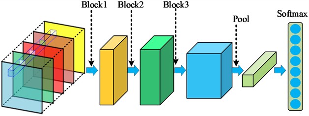
The role of the pooling layer in Fig. 1 mainly includes the following three aspects: 1) The pooling layer performs downwards sampling on the input data, reducing the spatial dimensions of the feature maps output by the convolutional layer. This procedure helps to decrease the number of parameters that need to be processed in the network, thereby lowering computational costs and the risk of overfitting. 2) The pooling layer enhances the ability of the model to learn translation invariance, increasing the robustness of the model to small translations in the input. 3) The pooling layer reduces redundant information in the feature maps, retaining more important features, which helps to extract more discriminative features. The fully connected layer is the terminal component in CNNs. When input data pass through multiple fully connected layers, the network gradually learns feature abstractions at different levels, ultimately mapping the network features to specific output categories or values. The neurons in the fully connected layer are connected to all the neurons in the previous layer. The calculation formula is as follows:

2

$\begin{array}{l}z=Wx+b,\\ a=f\left(z\right),\end{array}$

where $W$, $x$, $b$, and $z$ are the weight matrix, the input vector, the bias vector, the sum of the weighted input and bias, and the output of the activation function $f$, respectively. The convolutional operation, output, pooling layer, and fully connected layer calculations collectively constitute the basic framework of CNN.

3. Model building and experimental set-up

3.1. Experiment of bearing fault conditions

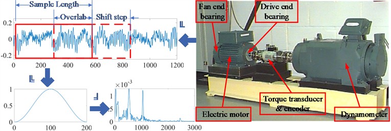
In this work, online data downloaded from the Case Western Reserve University Bearing Data Center website are employed for bearing fault diagnostic model training and testing. As shown in Fig. 2, there are three steps in the data acquisition process.

In the first step, experiments are conducted using a 2 hp Reliance Electric motor, and acceleration data are measured at locations near and remote from the motor bearings. In this work, data from a single accelerator sensor near the fan bearing position are used. During the experiment, bearings are first seeded with faults via electrodischarge machining (EDM). Fault sizes ranging from 0.007 inches to 0.040 inches in diameter are introduced separately at the inner raceway, rolling element (i.e., ball), and outer raceway. Faulted bearings are then reinstalled into the test motor, and vibration data are recorded for motor loads at different horsepower levels (motor speeds of 1797 to 1720 rpm) with a sample frequency of 12 kHz. In the second step, the obtained raw vibration signal in the time domain is scanned by a sliding Hanning window with a size of 600 and a shift step size of 400 to generate the raw signal samples. Therefore, for any two consecutive samples, there is an overlap of 200 data points. In the third step, the FFT spectrum of these vibration samples is calculated and employed as the input data for the diagnostic model.

Notably, five types of vibrations, namely, normal, inner raceway, outer raceway, ball element of the fan end bearing, and inner raceway of the drive end bearing, are considered in building the next model. All types of vibration signals are collected at motor speeds of 1772 rpm and 1730 rpm. For the faulty condition discussed in this work, the fault diameters are 0.007 inches and 0.014 inches.

Fig. 2Flowchart of bearing data acquisition

3.2. DS-CNN modelling process

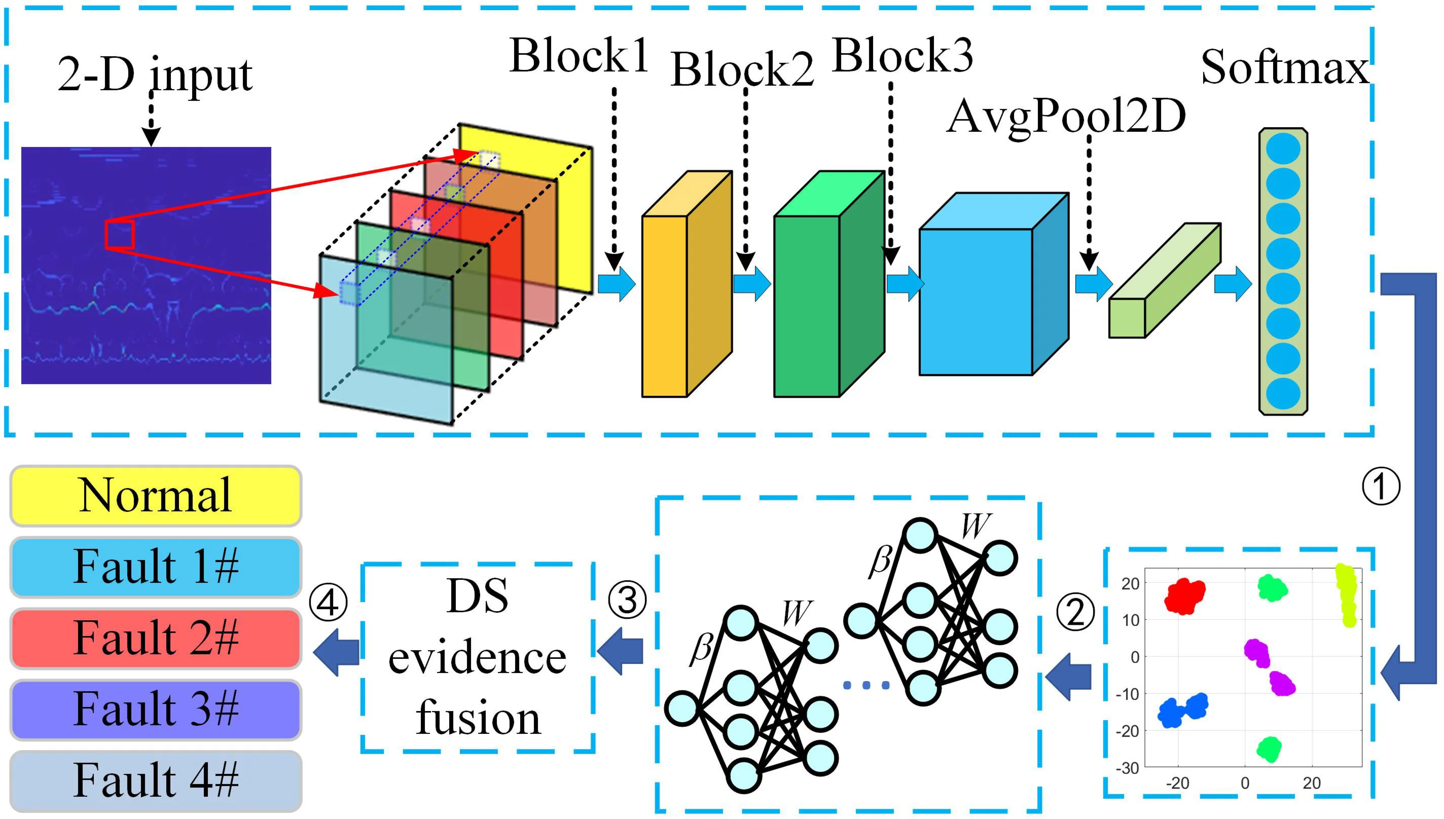
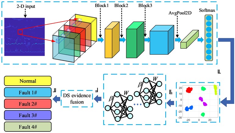
Multiple extreme learning machine modules are adopted as subclassifiers and fused via DS evidence fusion for fault diagnosis. The overall technical flowchart of the DS-ELM is shown in Fig. 3. There are four steps in the proposed diagnosis model, namely, signal processing, model training, model testing, and diagnostic evidence fusion.

In the first step, the vibration data are converted into a time-frequency image by the WSET. These time-frequency images are subsequently input into a two-dimensional CNN for adaptive fault feature extraction. The output result from the fully connected layer is used as the feature value of the vibration signal. In the second step, multiple neural network modules with different network parameters are employed as subclassifiers and independently trained on the training sample. In the third step, all subclassifiers produce raw diagnostic results from the testing sample. In the last step, a diagnostic evidence fusion process via DS evidence theory is performed for the final fault diagnosis output. Notably, for objective model evaluation, the average accuracy of the proposed technique needs to be tested, and multiple rounds of fault diagnosis are unavoidable. Taking one fault diagnosis round as an example, for each training process, the data samples in the training set need to be randomly selected from all the data samples each time. In addition, once the data samples are used for training, they should not be employed in model testing.

Fig. 3Process of DS-CNN-based fault diagnosis

4. Result analysis

For further model training and testing, the obtained signal eigenvalue is first divided into Dataset A and Dataset B as shown in Table 1. More specifically, in Dataset A, a represents a bearing fault size of 0.007 inches in diameter at a motor speed of 1730 rpm, and b represents a bearing fault size of 0.014 inches in diameter awt a motor speed of 1772 rpm. Therefore, if the model training and testing are conducted on Dataset A, 50 groups of vibration samples with a bearing fault size of 0.007 inches in diameter at a motor speed of 1730 rpm are randomly selected from Dataset A and employed for model testing in each training round (100 groups of vibration samples in total).

It worth mentioning that to ensure consistent and reliable results, the evaluation models are typically tested multiple times under identical conditions. Taking Dataset A from Table 1 as a reference, during each training iteration, all 50 data points in the training set must be randomly selected from Dataset A. The original testing set is then substituted with the remaining 50 unselected data points to form a new evaluation environment for subsequent iterations. This process guarantees that both training and testing datasets remain independent across different cycles, minimizing potential interference between them while ensuring fair performance assessment of each model instance.

Figs. 4 and 5 show the feature distributions of the vibration before and after the signal processing by the convolutional layers of the CNN. The vibration features exhibit greater separation after the adaptive extraction technique of the CNN. Separation is not easily distinguishable when the raw vibration data are input, whereas, after feature extraction by the CNN, these features become clearly divided in the fully connected layer.

Fig. 4Visualization of dataset A

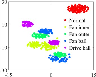
a) Original data distribution

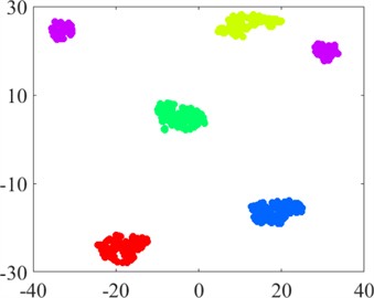
b) Data distribution after CNN

Fig. 5Visualization of dataset B

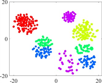
a) Original data distribution

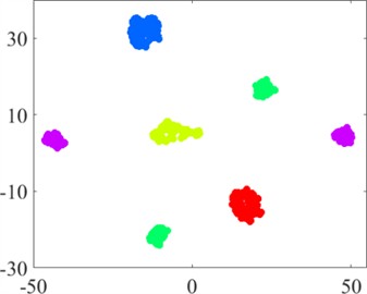
b) Data distribution after CNN

Notably, data features within the same fault category cluster into several groups, which are distributed in different locations. This separation occurs because each fault category contains five types of fault data. Although these data belong to the same fault category, the distinctive features between different fault data are relatively pronounced. Overall, the results indicate that our model can learn basic fault features from the raw vibration signal in an adaptive manner; thus, the model exhibits good adaptive feature extraction, which can increase the accuracy and robustness of bearing fault diagnosis.

In this paper, four types of fault diagnosis models built from individual back propagation neural networks (BPs), support vector machines (SVMs), extreme learning machines (ELMs), and echo state networks (ESNs) are compared. Tables 2 and 3 list the average accuracies of the diagnosis of each bearing fault by multiple classifiers. Notably, the overall diagnostic accuracy of each classifier in this paper is lower than those reported in previous studies with deep learning-based models. This difference can be explained by the fact that our training set contains relatively few samples, and only 50 groups of data samples are employed for model training. In cases of insufficient data, the model is prone to overfitting, and the model trained in the source domain experiences a significant drop in diagnostic performance in the target domain. This result indicates that the deep network structure has not truly learned the mapping relationship between vibration signals and bearing fault labels.

Fig. 6 illustrates the fault diagnosis accuracy of different classifiers over 100 test rounds. The accuracy of each individual model varies widely, indicating poor stability of the model. Taking the ESN model under Dataset B as an example, its highest diagnostic accuracy is 100 %, and the lowest is 38 %, resulting in an accuracy error of 62 %. Similar phenomena are also observed in the BP-based and ELM-based individual fault diagnostic models. In addition to overfitting, these large accuracy errors can also be caused by the fact that the network training process is prone to becoming stuck in local optimum values. In other words, if the parameters obtained through the model training approach reach the global optimum, the diagnostic accuracy will be high. Conversely, if the parameters only reach a local optimum, the diagnostic accuracy cannot be guaranteed.

Fig. 6Comparison of fault diagnoses by different classifiers

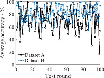
a) BP

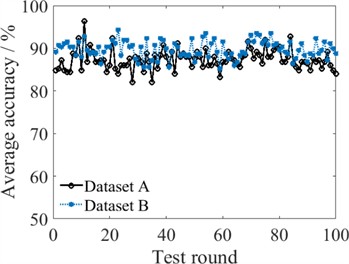
b) SVM

c) ELM

d) ESN

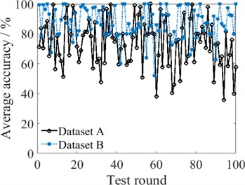
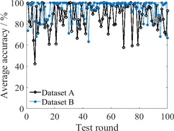
Notably, the fault diagnosis accuracy of the SVM exhibits the least variation, which is determined by the fault diagnosis mechanism of the SVM. In the process of fault diagnosis via SVM, features are first mapped into a specific space, and then a classification hyperplane is constructed in this space for direct data classification. During this process, fewer parameters (mainly the kernel parameter and the penalty parameter) affect the diagnostic accuracy of the model, and these two parameters do not require iterative training. The SVM has high diagnostic stability, but its model output is a classification hyperplane, which is not suitable for information fusion. The model output accuracy of the BP neural network is generally too low, which may reduce the accuracy of the final ensemble model. The ESN model already reaches an average accuracy of 94.22 on Dataset B. Therefore, the ELM module is used as a subclassifier in an ensemble fault diagnosis model utilizing DS evidence fusion. The related results are shown in Table 4 and Fig. 7.

Fig. 7Fault diagnosis comparison of individual and ensemble models

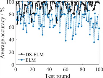
a) ELM under Dataset A

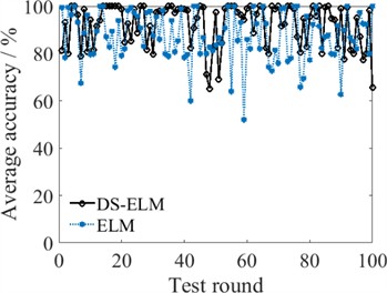
b) ELM under Dataset B

With DS evidence fusion, the average fault diagnosis accuracies of 100 test rounds are 92.06 % and 92.40 %, increasing from 74.05 % and 87.40 % for Dataset A and Dataset B, respectively. Moreover, the proposed ensemble model obviously enhances the stability of the bearing fault diagnosis. As multiple ELM modules are adopted as subclassifiers, the ensemble diagnostic model is more flexible and more suitable for addressing complicated fault diagnosis work since more ELM modules can be added to enhance the model’s ability to store more complex nonlinear mapping relationships. In addition, the ensemble model has stronger robustness. Even if some ELM modules suffer from strong disturbances and produce incorrect diagnostic outputs, the correct result is still likely to be obtained through fusion analysis. However, the main limitations of our model come from two aspects. One limitation is the issue of unbalanced input, it is not analyzed currently. Another limitation is the efficiency problem. Multiple modules mean more training time than individual models to a certain degree. In future, more advanced optimization algorithms will be analyzed to further enhance the ensemble model. In summary, the ensemble diagnostic model exhibits good performance in terms of diagnostic accuracy and stability for bearing fault diagnosis.

5. Conclusions

In this paper, a new ensemble model called DS-ELM consisting of multiple ELM modules and utilizing DS evidence fusion theory is proposed. The novel model does not rely heavily on expert prior knowledge for fault feature extraction since it is completed adaptively by a CNN. Multiple ELM modules are employed to build the ensemble model, and its diagnostic accuracy can be guaranteed when trained with a small sample size since it is a shallow neural network that has fewer network parameters than a deep learning-based model. Through fusion analysis, the final ensemble model addresses the fact that individual models easily become stuck in local optima during the training process, leading to poor model accuracy for fault diagnosis. On the other hand, as the ensemble model can produce comprehensive results from multiple ELM modules, its diagnostic performance is not sensitive to the network parameters of a specific ESN module. In addition, even if the result of a specific module is not satisfactory, the overall output of bearing fault diagnosis will not be affected, which enhances model robustness. In future work, more optimization investigation of the reported ensemble model will be conducted to improve its bearing fault diagnostic performance and further explore its capability for more complex fault diagnosis tasks.