Application of laser scanning for automated efficiency assessment of solar panels: a case study in Uzbekistan

1. Introduction

Solar energy is one of the most dynamically developing sectors of renewable energy [1, 2]. In the face of global climate change and rising energy consumption, countries are striving to utilize environmentally friendly energy sources. One key area of this process is the implementation of photovoltaic (PV) systems [3, 4].

The efficiency of solar panels depends on many factors: solar insolation, regional climate, the quality of the photovoltaic cells, and, most importantly, the panel tilt angle [3, 5]. For Uzbekistan, and particularly for Tashkent, solar energy has enormous potential. According to statistics, the country receives over 250 sunny days per year, and the average annual solar radiation level exceeds 1,600 kWh/m² [6]. This makes the republic one of the leaders in Central Asia in terms of solar power plant development potential [7].

There are a few commonly used approaches to determining the tilt angle of solar panels. The first approach is based on empirical formulas that assume the best tilt angle equals the location's latitude ±10-15° [5], [8]. The second approach is based on experimental observations, and the angle is selected based on long-term meteorological observations [9]. The third approach is based on mathematical modeling and predictions of the sun’s location by using geometric and physical models of solar motion [1], [3], [6].

In addition, recent comparative analyses of fixed-tilt and tracking PV systems show that tracking configurations can improve annual energy yield by 15-25 %, depending on latitude and climatic zone [9], [10]. However, these systems are more expensive and require complex maintenance, so determining the optimal fixed tilt angle remains an important engineering task [10], [11].

The cost-benefit analysis, based on a review of the existing literature, is as follows. Based on the review of [9, 10, 16, 17], tracking systems are a sound investment in sunny regions – typically delivering 20-30 % more electricity output and lower lifetime cost per kWh than fixed-tilt systems. Based on [9, 16], single-axis trackers are the best value: simpler, cheaper, and close to dual-axis performance. They are widely used in utility-scale plants worldwide. In contrast, dual-axis trackers may suit special cases but are not cost-effective in general. It is well-known that solar panels become less efficient when their temperature exceeds a certain threshold. While solar panel cooling systems, such as spray-water designs, are possible and show promise in lab conditions, they are impractical for large-scale desert use without water recycling. In addition, cost-benefit analysis should include: (1) full-year performance data (not just day-level), (2) downtime and stow losses, (3) soiling and cleaning costs, (4) bifacial modules and reflective ground effects, and (4) hourly energy pricing and curtailment. When these are added, the realistic financial benefit of tracking typically equals 15-25 % more net revenue, rather than the optimistic 30 % headline.

This study focuses on one PV system installation in the New Uzbekistan area of Tashkent (Uzbekistan). Geographical and climatic Features of Tashkent are as follows: Tashkent is located at a latitude of 41.31°N and a longitude of 69.28°E. The time zone is UTC+5. A distinctive feature of the region is its pronounced continental climate. In winter, the sun rises low on the horizon, so the panels must be tilted at a steep angle to capture the sun’s rays at right angles. In summer, on the contrary, the sun is high, and the panels must be positioned closer to the horizontal. It is worth noting that there are many roof-installed PV systems in Uzbekistan, and the majority of them are fixed-axis.

The main objective is to assess the efficiency of a typical PV system installation in Tashkent and to propose improvements if deficiencies are identified. The angular orientations of the solar panels in space were obtained by using a terrestrial laser scanner.

2. Point cloud of the solar panels

2.1. Laser scanning of a building block

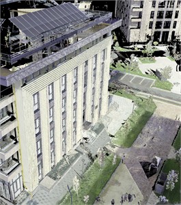
As part of a large-scale efficiency assessment project of solar panels installed on the rooftops of several buildings, a set of newly constructed buildings in the New Uzbekistan area of Tashkent was laser-scanned. The laser scanning project was conducted on September 15, 2025, and included a few buildings around a small square. The terrestrial laser scanner RTC360 [12] from Leica Geosystems was used in this study. The scanning was conducted from multiple stations, and the final registration of the point clouds collected from different stations was done in Cyclone Register 360+ software package [13], also from Leica Geosystems. The resultant point cloud is shown in Fig. 1, with the intensity colors of the returned laser beam.

Fig. 1Point clouds of newly constructed buildings with solar arrays on top

3. Point cloud of solar panel array and its analysis

One of the main objectives is to develop an approach for automated, mass-scale efficiency analysis of solar panel arrays based on the calculation of panel orientation from a laser scanner. As shown in Fig. 1, all the buildings have solar panels on their rooftops.

To demonstrate the developed approach, only one building was considered in this study. The point cloud of the building with an array of solar panels on top is shown in Fig. 2.

Fig. 2Point cloud of the selected building

a) Isotropic view

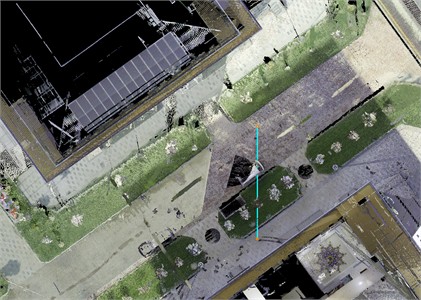
b) Plan view with $X$-axis shown (blue line)

Based on the measurements conducted at the site, the building’s south wall is oriented at 54 degrees to the north-east. The point cloud coordinate system was adjusted accordingly, and the resulting coordinate system is shown in Fig. 2(a) and Fig. 2(b). The latter images show the point cloud colored with the natural colors collected by the still-imaging camera built into the scanner.

Fig. 2(b) shows the $X$-axis of the new coordinate system, introduced to align it with magnetic north. In this plan view image, the $X$-axis is shown as a blue line, and its upward direction points north.

The point cloud of the solar panel array, isolated from the rest of the building, is presented in Fig. 3(a).

Fig. 3Analysis of the point cloud of the solar panel array

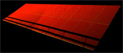
a) Point cloud of the solar panel array

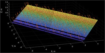
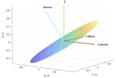
b) Normals to the point cloud of the solar panel array

The point cloud of the solar panel array was analyzed in MATLAB [14] environment. The normals to the point cloud were computed as shown in Fig. 3(b). This image was obtained as a result of the following. First, the point cloud was down-sampled to achieve an even point distribution. Second, a special MATLAB function that uses several neighboring points to generate a normal to the surface was used. In this paper, a hundred neighboring points were used. The degree of down-sampling and the number of neighboring points can be adjusted based on the point cloud's density.

Due to an error in acquiring the point clouds and some reflectivity-related issues, the point cloud contained some noise. All three components were checked for variability, and the coefficient of variability (COV) was calculated for each component. The COV is the ratio of the standard deviation to the mean expressed as a percentage. It was determined that the first component has a COV of 2.9 %, the second component has a COV of 3.8 %, and the third component has a COV of 1.0 %. Since the COV did not exceed 45 for all three components, this variability was considered acceptable.

The angles of a normal vector with respect to the reference $X$-axis and $Z$-axis were obtained by computing the dot product (scalar product) of the normal vector with the unit vector of the respective axis, namely (1,0,0) and (0,0,1). These computations were conducted for the average values of $X$, $Y$, and $Z$ components of the normal vectors. The results reveal that the angle to the $X$-axis is –144.2 degrees. In contrast, the normal inclination with respect to the vertical axis is 59.1 degrees, as presented in Fig. 4(a). This image also shows a round portion of the solar panel in the middle of the array where the origin of the coordinate system was selected.

Fig. 4The panel’s normal and angular coordinates of the sun’s location

a) The panel’s normal in the selected coordinate system with a round portion of the panel

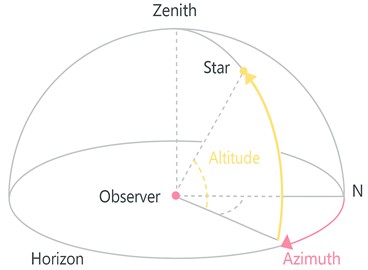
b) The angular coordinates of the sun’s location

The angular coordinates of the sun’s location are shown in Fig. 4(b). Information on the sun’s angular coordinates is widely available, including a few online calculators (see [15] as a representative example).

As an example, the change of the sun’s location on the day of scanning, September 15, 2025, is presented in Fig. 5(a). This data was taken from [15] for the geo-location of the scanned site.

Fig. 5The angular coordinates of the sun’s location on 09/15/2025 and their vector representation

a) The angular coordinates of the sun’s location at the scanned site on 09/15/2025

b) The normal to the solar panel array (cyan) compared to the sun directions (black) on 09/15/2025

In the coordinate system of the sun depicted in Fig. 4(b), the azimuth of the solar panel is 144.2 degrees, and the altitude is 30.9 degrees (which is a result of subtracting 59.1 degrees from 90 degrees).

For this particular day, the normal of the solar panel array has a higher altitude than the maximum value of the sun’s altitude, as shown in Fig. 5(b). In this figure, the sun directions on the day of scanning are shown as black arrows with 15-minute intervals.

To conduct a comparative study of the efficiency of this actual installation and potential modifications, four models were introduced, as listed in Table 1. It is worth noting that modifications PVS2 and PVS3 may result in a reduction in square footage. For simplicity of the discussion, this is ignored in this study and will be investigated in future research.

For PVS1 and PVS2, the normal to the solar panel array will vary throughout the day, as shown in Fig. 6(a), because each is a single-axis system. In contrast, PVS0 and PVS3 are fixed-axis systems, and as such, their normals remain fixed throughout the day.

Fig. 6The normals of all PV models and the resultant cosine function

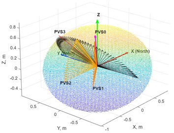
a) The normals of all models compared to the sun directions (black) on 09/15/2025

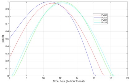
b) The variation of this cosine function with time (as an example, the day of scanning is shown)

The angle between the sun’s direction and the normal to the solar panel array, $\theta$, determines the array’s power output, $P$:

The cosine of this angle can be obtained from the dot product (scalar product) of the unit normal vector, $N_{panel}$, and the unit vector pointing to the sun’s current location, $N_{sun}$:

From Eq (1), we can obtain that the variation of this cosine with time is the same as the variation of power over time, normalized by $P_{max}$:

This power variation over time is shown in Fig. 6(b). It is worth noting that the cosine can become negative, corresponding to cases when the sun is below the solar panel; as such, for these cases, the cosine is assumed to be zero.

Based on Eq. (3), the sum of all cosine variations throughout a day multiplied by the $P_{max}$ will result in the power output of the solar panel. Therefore, this daily power output can be normalized by dividing by $P_{max}$, as shown in Fig. 7(b) for the same day. This image shows the cumulative sums of power output over time.

Fig. 7The variation of this normalized power output with time (as an example, the day of scanning is shown)

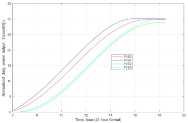
a) The variation of the normalized power output with time on 09/15/25

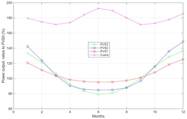
b) Ratio of daily power outputs for all models

It is worth noting that the last number on the right side of each plot corresponds to the normalized daily electricity production, $E_d$/$P_{max}$, when multiplied by the time increment, $dt$ (0.25 hours, which corresponds to 15 minutes), as presented below:

Plots similar to those presented for the day of laser scanning were generated for each month of 2025. The 15th day of each month was selected for that. All data were obtained from [15]. These daily power outputs were divided by those for the model PVS0, and the resulting ratios are presented in Fig. 7(b). As shown, all models with modifications to the current installation are more effective in the spring and fall months.

The numbers depicted in Fig. 11 were assumed to represent average monthly power outputs, and when multiplied by the number of days in each month, they produced the results shown in Table 2.

The latter table shows that the current orientation and the fixed-axis configuration of the solar panel system are quite effective, as the system’s production is close to that of all modified versions. The most effective one is the single-axis system oriented south. It is worth noting that the difference in the energy output is less dramatic than was expected from the cost-benefit analysis. It is related to the fact that all these systems are idealized, and losses due to increased construction costs, actuator, controller, and other expenses are not yet accounted for. This will be done in the future extended study.

4. Conclusions

This article presents an approach for automated assessment of the efficiency of pre-installed solar panel arrays. It is based on the utilization of the laser scanner. The approach allows evaluating deficiencies in power production efficiency and comparing them with cost-effective modifications. The cost-benefit analysis can be performed based on this assessment.