Abstract
To accurately predict the remaining useful life (RUL) of rolling bearings under strong noise interference, this paper proposes an RUL prediction method based on adaptive Variational Mode Decomposition (VMD) and a hybrid Temporal Convolutional Network-Gated Recurrent Unit-Self-Attention (TCN-GRU-SA) framework. First, a parameter-optimized VMD algorithm is developed by integrating the Grey Wolf Optimizer (GWO) with VMD to extract effective intrinsic mode components (IMFs) and reconstruct denoised signals, thereby mitigating the impact of strong background noise. Subsequently, time-domain degradation features are extracted from the reconstructed signals to generate more representative feature datasets. These degradation features are then fed into a parallel TCN-GRU-SA prediction model. To enhance the model’s generalization capability and RUL prediction performance, the proposed hybrid architecture combines a Temporal Convolutional Network (TCN), which captures local temporal patterns, a Gated Recurrent Unit (GRU) for modeling long-term dependencies, and a Self-Attention (SA) mechanism to prioritize critical degradation-related features. Experimental validation on the PHM2012 rolling bearing accelerated lifetime dataset demonstrates that the proposed method achieves superior noise robustness and prediction accuracy compared to existing approaches. Specifically, it reduces the root mean square error (RMSE) by 18.7 % and improves the coefficient of determination (R2) by 12.3 % under high-noise conditions, confirming its effectiveness in industrial predictive maintenance applications.
Highlights
- An adaptive GWO-VMD method with weighted kurtosis is proposed for automatic parameter selection and robust noise suppression.
- A parallel TCN-SA and GRU-SA dual-branch framework is constructed to extract complementary multi-scale features and dynamic temporal evolution.
- Self-attention mechanisms are integrated to dynamically reinforce critical fault features and reduce noise interference for higher accuracy.
1. Introduction
In modern industrial applications, rolling bearings are ubiquitous components of rotating machinery, where their operational integrity is paramount for equipment efficiency and safety. Subjected to prolonged service under harsh operating conditions, bearings are prone to degradation. As detailed in existing literature on dynamic fault modeling [1], failure modes typically manifest as spalling, cracks, wear, plastic deformation, and pitting. Because distinct local and distributed faults exhibit disparate dynamic signal characteristics, they present unique challenges for health monitoring. This study specifically targets the degradation processes driven by fatigue spalling and continuous wear – the dominant factors limiting service life in accelerated aging scenarios. Consequently, precise Remaining Useful Life (RUL) estimation under these conditions is critical for minimizing downtime and optimizing maintenance strategies [2-4].
RUL prediction methodologies are generally categorized into physics-based and data-driven approaches [5-7]. Physics-based methods leverage an in-depth understanding of failure mechanisms to construct mathematical models of the degradation process [8]. Theoretically, these models characterize intrinsic system dynamics [9]. However, because bearing faults within complex systems involve the coupling of multiple physical fields, the underlying damage evolution mechanisms remain partially obscure [10], hindering the construction of high-precision physical models.
Conversely, data-driven methods, which rely on the volume and quality of monitoring data rather than extensive prior expert knowledge, have gained significant traction. While conventional algorithms such as Support Vector Machines (SVMs) [11] and Artificial Neural Networks (ANNs) [12] yield acceptable results in controlled settings, they often struggle with high-noise interference and complex non-linear relationships inherent in large-scale industrial datasets. To address this, deep learning architectures have been widely adopted. For instance, Yang et al. [13] and Ding et al. [14] utilized Convolutional Neural Networks (CNNs) for feature extraction. However, while CNNs excel at capturing local spatial features, they are less effective at modeling long-term temporal dependencies. To bridge this gap, hybrid architectures have emerged: Luo et al. [15] combined CNNs with Bidirectional Long Short-Term Memory (Bi-LSTM) networks, Liu et al. [16] integrated deep CNNs with Bidirectional Gated Recurrent Units (BiGRU) and Self-Attention (SA) mechanisms, and Cao et al. integrated the Temporal Convolutional Network (TCN) with the Transformer [17]. Despite these advancements, accurate RUL prediction under conditions of strong noise and limited sample sizes remains a persistent challenge.
To overcome these limitations, this paper proposes a novel RUL prediction framework utilizing adaptive Variational Mode Decomposition (VMD) and a parallel hybrid neural network. First, to mitigate background noise, we develop a parameter-optimized VMD algorithm using the Grey Wolf Optimizer (GWO) to adaptively extract effective Intrinsic Mode Functions (IMFs). Second, we design a hybrid model combining a Temporal Convolutional Network (TCN), Gated Recurrent Unit (GRU), and Self-Attention (SA) mechanism to extract complementary degradation features.
The main contributions of this work are as follows:
1) A noise-robust signal processing method (GWO-VMD) is proposed. By integrating the Grey Wolf Optimizer with VMD, this approach eliminates the subjectivity of manual parameter tuning found in traditional VMD. Incorporating a weighted kurtosis criterion enables the adaptive selection of optimal decomposition parameters, effectively isolating fault signatures from noise. This yields significant noise suppression and superior feature quality compared to fixed-parameter approaches.
2) A parallel TCN-GRU-SA dual-branch hybrid model is constructed for RUL prediction. This architecture exploits the complementary nature of heterogeneous features: the TCN branch captures multi-scale local and global trends via dilated convolutions, while the GRU branch models the dynamic evolution of temporal sequences. Furthermore, the SA mechanism dynamically weights features to emphasize critical degradation indicators while suppressing irrelevant interference, thereby enhancing prediction accuracy and robustness.
2. Theoretical background
2.1. VMD
Variational Mode Decomposition (VMD) is a non-recursive signal decomposition technique proposed by Dragomiretskiy and Zosso [18]. Unlike the recursive sieving of Empirical Mode Decomposition (EMD), VMD decomposes a real-valued input signal into a discrete number of band-limited Intrinsic Mode Functions (IMFs), denoted as . Each mode is compact around a central frequency .
The decomposition is formulated as a constrained variational optimization problem, aiming to minimize the sum of the estimated bandwidths of each mode while reconstructing the original signal. This problem is solved efficiently using the Alternating Direction Method of Multipliers (ADMM) algorithm. The detailed mathematical derivation and the iterative update steps for and can be found in the original literature [18].
In practical applications, the performance of VMD relies heavily on two pre-set parameters: the number of modes and the penalty factor (bandwidth control parameter).
The number of modes : An improper value leads to either mode mixing (under-segmentation) or the generation of spurious components (over-segmentation).
The penalty factor (): This parameter determines the bandwidth of the decomposed modes. A smaller retains more information but allows more noise, while a larger effectively suppresses noise but may filter out useful fault features.
Since these parameters are signal-dependent and lack a universal selection standard, determining the optimal combination of is critical for accurate fault feature extraction. This necessitates the use of the adaptive optimization method proposed in the following section.
2.2. GWO-based adaptive VMD method
Inspired by the hunting behavior of gray wolf packs, Mirjalili et al. [19] proposed the Grey Wolf Optimizer (GWO) in 2014. This algorithm simulates three key phases of gray wolf hunting – searching for prey, encircling and chasing prey, and attacking prey – to achieve optimal search performance. Compared to other optimization algorithms, the GWO features a simple structure, fast convergence speed, and a balance between local and global optimization. It also incorporates an information feedback mechanism, requires fewer parameters, and exhibits strong robustness, making it widely applicable across various fields. In this paper, the GWO is integrated with VMD to propose a parameter-adaptive VMD method based on the GWO. The algorithmic workflow is as follows:
1) Select the envelope entropy as the fitness function, which is defined as follows:
where, represents the envelope signal sequence obtained by applying Hilbert demodulation to the signal , and is the normalized form of . denotes the Hilbert transform of the signal. Envelope entropy serves as a measure of the sparsity of the original signal. For an Intrinsic Mode Function (IMF) dominated by noise components with limited feature information, the envelope entropy value tends to be higher. Conversely, if an IMF contains rich feature information and fewer noise components, the envelope entropy value will be lower. Therefore, minimizing the envelope entropy is essential to enhance denoising performance and retain more useful feature information.
2) Set the search ranges for parameters and , initialize a population by randomly generating candidate solutions , input the original signal into the algorithm, and perform iterative optimization based on the fitness function proposed in this study.
3) Upon completion of the iteration, the optimal parameters are substituted into the VMD to perform signal decomposition, thereby obtainingIMF components.
4) An effective weighted kurtosis index [20] is introduced to screen the components, and the selected effective modal components are reconstructed to mitigate the interference of strong background noise.
2.3. Model construction
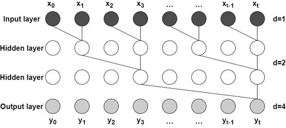
The Temporal Convolutional Network (TCN), introduced by Bai et al. [21], represents a specialized architecture tailored for sequence modeling. In contrast to Recurrent Neural Networks (RNNs), the TCN leverages dilated causal convolutions and residual connections to process time-series data efficiently. Its architecture is defined by three core components:
Causal Convolution: This mechanism ensures strict temporal ordering, where the prediction at time depends exclusively on historical data , thereby preventing any information leakage from future states.
Dilated Convolution: By inserting gaps between kernel elements, this technique enables the network to exponentially expand its receptive field without increasing the parameter count. This allows the model to effectively capture long-term dependencies inherent in bearing degradation signals.
Residual Blocks: These structures facilitate the training of deep networks by mitigating the vanishing gradient problem. In this study, the TCN is employed to extract high-dimensional temporal features from bearing vibration signals in parallel, ensuring high computational efficiency. The structure of the dilated causal convolution is illustrated in Fig. 1.
Fig. 1Dilated causal convolution
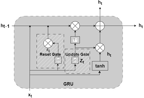
The Gated Recurrent Unit (GRU) is a streamlined variant of the Long Short-Term Memory (LSTM) network, developed to address the vanishing gradient problem prevalent in standard RNNs [22]. As depicted in Fig. 2, the GRU architecture simplifies the cell structure by synthesizing the input and forget gates into a single update gate, while utilizing a reset gate to modulate the flow of information. This gating mechanism enables the GRU to selectively retain critical historical information while discarding irrelevant noise, rendering it highly effective for modeling the sequential evolution trends of bearing degradation. Furthermore, compared to LSTM, the GRU’s reduced parameter complexity fosters faster convergence during training while maintaining comparable predictive performance.
Fig. 2GRU model internal structure
To further enhance the model’s ability to focus on critical degradation features, the Self-Attention (SA) mechanism is incorporated, as depicted in Fig. 3. Unlike TCN and GRU, which process data sequentially or locally, SA calculates global dependencies by computing the pairwise relationships between all elements in the sequence. Through the Query-Key-Value (Q-K-V) computation, SA dynamically assigns higher weights to time steps containing significant fault impulses and suppresses irrelevant background noise. This mechanism allows the model to prioritize the most informative segments of the vibration signal, thereby improving the robustness and accuracy of RUL prediction under complex operating conditions.
Fig. 3Self-attention convolution
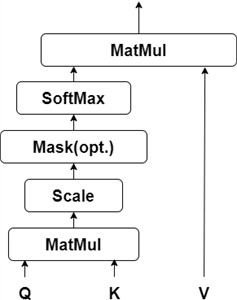
In the TCN branch, the Self-Attention (SA) mechanism applies cross-channel and temporal joint attention allocation (via Multi-Head Attention) to the convolutional feature maps. This approach enhances the global contributions of fault features – such as specific frequency components – while suppressing noise-dominated time segments, thereby improving the signal-to-noise ratio of the extracted features. Meanwhile, in the GRU-SA branch, the SA mechanism directly computes association weights across all time steps without being constrained by sequence length, enabling context-aware reweighting of the hidden-state sequence produced by the GRU and preserving key historical states (e.g., the initial healthy baseline). Furthermore, by identifying abnormal time points in real time through the attention weights, the SA mechanism can mitigate the GRU’s response lag when facing sudden transient events, such as the instantaneous impact of local bearing spalling.
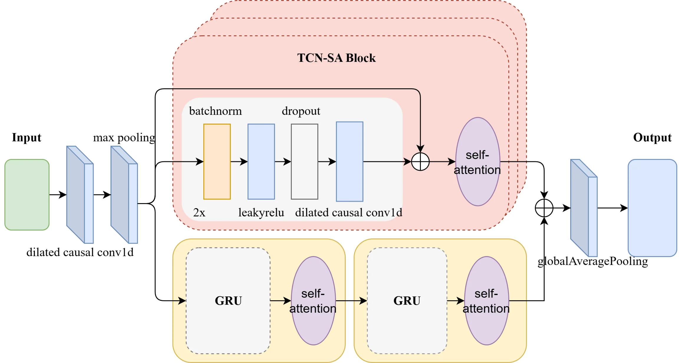
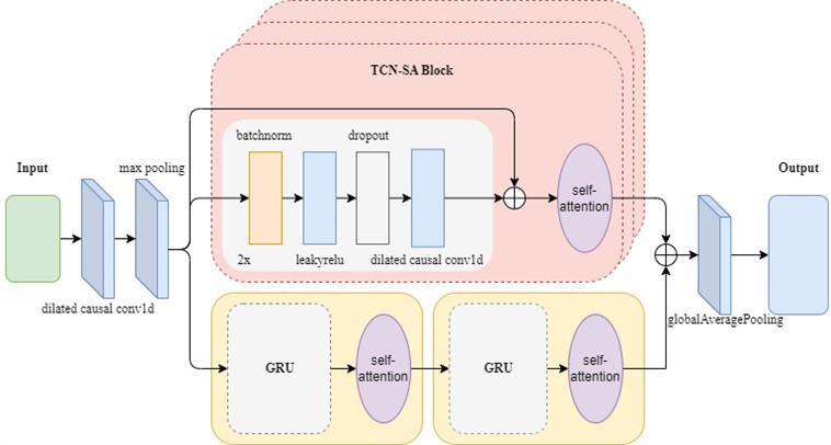
The Temporal Convolutional Network (TCN), Gated Recurrent Unit (GRU), and Self-Attention (SA) mechanism are integrated to construct a hybrid prediction model, termed the TCN-SA and GRU-SA Combined Prediction Model, as illustrated in Fig. 4. The network input is a 2D tensor derived from horizontal vibration sensor data. The input tensor undergoes a dilated one-dimensional convolution followed by max pooling, after which it splits into two parallel pathways: the TCN-SA branch and the GRU-SA branch. The TCN-SA branch consists of multiple stacked TCN modules and SA modules, where the TCN modules employ LeakyReLU activation functions to enhance robustness during parameter optimization [23], and the SA modules adaptively focus on critical features across time series, reinforcing long-range dependencies and amplifying the influence of pivotal information on predictions. The GRU-SA branch utilizes the GRU to model temporal dynamic evolution patterns and employs the SA mechanism to perform context-aware reweighting of hidden-state sequences, alleviating the long-term dependency decay inherent in traditional RNNs. The two branches are designed to exploit complementary strengths: TCN-SA prioritizes multi-resolution local-global feature fusion, capturing both fine-grained and coarse-grained temporal patterns, while GRU-SA focuses on continuous-state transition modeling, preserving temporal coherence in sequential data. Outputs from both branches are aggregated through a global average pooling layer, achieving multi-granularity feature fusion. The fused features are processed through the global average pooling layer to generate the final prediction, effectively reducing the number of trainable parameters and mitigating overfitting. This architecture synergizes the advantages of parallelized multi-scale feature extraction and sequential dynamics modeling, enabling robust and accurate RUL prediction under noisy industrial conditions.
Fig. 4Architecture of network model
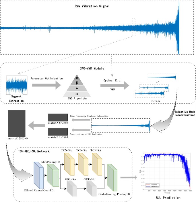
The TCN-GRU-SA model proposed in this study achieves rolling bearing lifespan prediction through the technical framework illustrated in Fig. 5. The key steps of the framework include the following:
1) GWO-Based Parameter-Adaptive VMD Method: A Grey Wolf Optimizer (GWO)-driven parameter-adaptive Variational Mode Decomposition (VMD) method is employed to select effective IMFs for signal reconstruction, thereby mitigating interference from strong background noise.
2) Time-Frequency Feature Extraction and Label Design: Multiple time-frequency domain features are extracted from the reconstructed signals, and prominent features are selected to form the input dataset. The Root Mean Square (RMS) value is utilized to design labels for the rolling bearing feature dataset.
3) Construction of the TCN-GRU-SA Model: A hybrid TCN-GRU-SA model is constructed, integrating the Temporal Convolutional Network (TCN), Gated Recurrent Unit (GRU), and Self-Attention (SA) mechanism.
4) Dataset Partitioning: The dataset is divided into training and testing sets, where the training set is used for model training and the testing set validates prediction accuracy.
5) Performance Evaluation Platform: To assess the effectiveness of the proposed method, an evaluation framework is constructed, incorporating metrics such as Root Mean Square Error (RMSE) and the coefficient of determination ().
2.4. Experimental dataset construction
2.4.1. Raw data
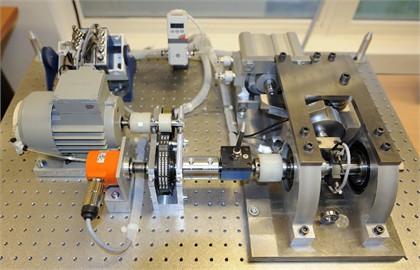
To validate the performance of the proposed lifespan prediction method, experiments were conducted using the publicly available dataset from PHM2012 (the PRONOSTIA accelerated aging platform) [24]. The experimental dataset is derived from the IEEE 2012 PHM Data Challenge and consists of vibration acceleration measurements. Each signal contains 2560 samples, collected every 10 s at a sampling rate of 25.6 kHz. The experimental setup is depicted in Fig. 6. In total, vibration data from 17 rolling bearings under three load conditions are available. For this study, the analysis focused on horizontal-direction bearing signals obtained at a rotational speed of 1800 r/min under a 4000 N load.
Fig. 5Technical roadmap
Based on measurements from the PHM2012 rolling bearing dataset under identical operating conditions, the vibration signals from Bearing 1-1 and Bearing 1-2 were identified as the most representative, as they comprehensively cover the majority of degradation states during bearing operation under the same conditions. Consequently, Bearing 1-1 and Bearing 1-2 were chosen as the training set, while Bearing 1-3, 1-4, 1-5, 1-6, and 1-7 were allocated to the test set.
To assess the predictive accuracy of the remaining useful life (RUL) estimation method, the RMSE and MAE are employed as evaluation metrics. Their mathematical formulations are given by:
where, denotes the actual RUL, represents the predicted RUL, and is the total number of test samples.
Fig. 6PRONOSTIA test platform
2.4.2. RUL label construction
In bearing RUL prediction, RUL labels are typically constructed in a linear form ranging from 1 to 0, as shown in the following formula:
where, represents the total lifespan of the rolling bearing, and denotes the time corresponding to the th data sample. Although the linear RUL labeling method is straightforward, it fails to effectively capture the nonlinear degradation characteristics of bearings, particularly during the early healthy phase and the accelerated degradation phase near failure.
The Root Mean Square (RMS) of vibration signals is adopted as a health indicator to design RUL labels, as it effectively captures the average energy of the signal and reflects the bearing’s degradation trend. The RUL labels are constructed by normalizing the RMS sequence and mapping it to a range from 1 (healthy state) to 0 (complete failure). The method for calculating RMS is as follows:
The RMS value is calculated using the formula above, where denotes the amplitude of the th data point in the vibration signal, and is the total number of data points in the sample. This value serves as a key feature for characterizing the bearing’s health state.
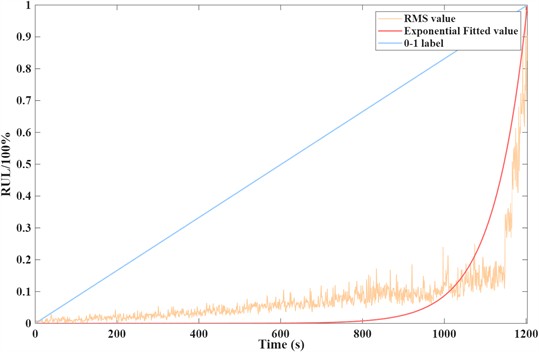
To clearly illustrate the impact of the RMS in characterizing the degradation trend of bearing performance, the variation in the RMS and the 0-1 linear value over time for Bearing1-1 are shown in Fig 7. As depicted, the RMS is influenced by multiple factors and does not exhibit a monotonic change over time. Therefore, to align with the monotonicity requirement of RUL labels, the RMS values are first fitted using an exponential function, and then the fitted values are normalized to the range of 0 to 1. The normalization formula is as follows:
where, is the normalized RMS value, and are the maximum and minimum values of the RMS, respectively. It can be observed that, compared to the 0-1 linear values, the normalized RMS values better characterize the degradation trend of the bearing. The slope of the normalized RMS curve can be used to indicate the degree of damage between adjacent time points, reflecting the transition from the normal state to the initial damage state and finally to the complete failure state.
Fig. 7Change trend of RMS over time
3. Results and discussion
3.1. GWO-VMD experiments and performance comparison
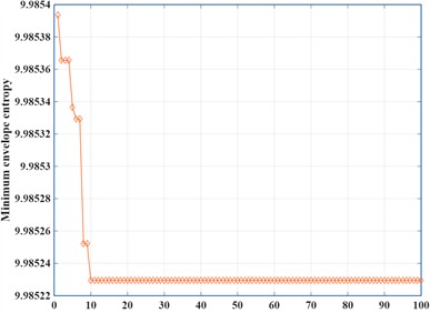
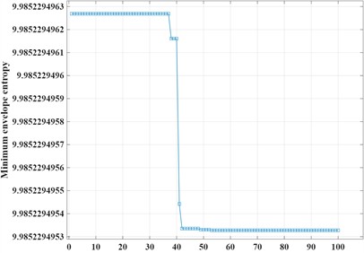
To demonstrate the superior performance of the Grey Wolf Optimizer (GWO) algorithm in terms of optimization speed and precision, Fig 8 compares the optimization effects of Particle Swarm Optimization (PSO)-VMD and GWO-VMD on parameters and . The GWO algorithm exhibits faster convergence during the iterative process, achieving a minimum envelope entropy value of 9.98523 after 10 optimization runs (Fig. 8(a)). In contrast, the PSO algorithm requires 49 iterations to converge, ultimately yielding a slightly lower minimum envelope entropy value of 9.98522 (Fig. 8(b)).
Fig. 8Optimizing results
a) GWO iterations
b) PSO iterations
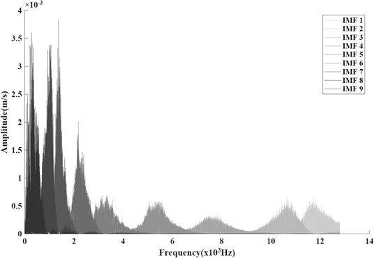
Following the algorithmic steps described in Section 2.2, the envelope entropy was selected as the fitness function, with the search ranges for parameters and set to [3, 10] and [1000, 3000], respectively.For the configuration, the population size was set to = 2, the spatial dimension to dim = 2, and the iteration limit to = 100. Ultimately, the optimal position of the gray wolf population is [9, 2425], it was found that the best values for and are 9 and 2425, respectively, and the frequency-domain decomposition of Bearing1-1 is presented in Fig 9. As illustrated in Fig. 9, the GWO-optimized adaptive VMD algorithm successfully decomposed the vibration signal into nine IMFs, effectively separating the frequency components with minimal mode mixing or under-decomposition. Subsequently, the effective weighted kurtosis of each IMF component was calculated, and components with positive weighted kurtosis were selected for signal reconstruction based on the effective weighted kurtosis criterion.
Fig. 9Bearing1-1 frequency domain decomposition results
The noise reduction performance of the proposed approach was evaluated by comparing the GWO-optimized adaptive VMD algorithm with EMD and VMD. The Root Mean Square Error (RMSE) between the reconstructed and true signals was adopted as the criterion for measuring denoising effectiveness. In addition, the RMSE of the Bearing1-1 vibration signal was analyzed across different SNR levels, as illustrated in Fig. 10.
Fig. 10RMSE of Bearing1-1 under different SNR conditions
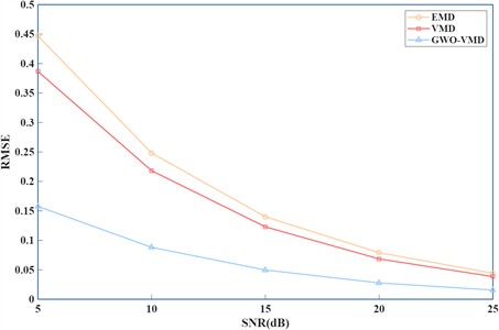
As shown in Fig. 10, the RMSE gradually decreases as the SNR increases. Compared to the EMD and VMD algorithms, the proposed denoising algorithm consistently exhibits lower RMSE values. This superior performance is attributed to the integration of the GWO, which combines high-precision global search capability and rapid convergence, to adaptively determine the optimal values of parameters (number of modes) and (penalty factor). Furthermore, under strong noise interference, the proposed algorithm demonstrates significant advantages over traditional VMD. This is because the algorithm not only adaptively optimizes and , but also employs the effective weighted kurtosis criterion to filter out informative IMFs, thereby achieving more accurate signal reconstruction. The comparative results confirm that the GWO-optimized adaptive VMD algorithm possesses stronger denoising capabilities.
3.2. RUL experiments and performance comparison
According to the algorithmic steps described in Section 2.3, the parameters used by the model for the PHM2012 dataset are listed in Table 1.
Table 1Network parameters
Layer | Parameters |
Dilated causal conv1d | filters = 8, kernel = 32, stride = 4 |
Maxpool1d | Pool size = 4 |
TCN-SA1 | filters = 3, kernel = 16, dilation = 1 |
TCN-SA2 | filters = 3, kernel = 32, dilation = 2 |
TCN-SA3 | filters = 3, kernel = 64, dilation = 4 |
Dropout | rate = 0.4 |
In the branch structure of the TCN-SA network, small convolutional kernels are employed in the convolutional layers to reduce the training burden of the model. The number of channels is set as multiples of 16 and gradually increases. The stride determines the downscaling ratio of feature dimensions after downsampling. The dilation rates, which control the expansibility of dilated convolutions, are set to 1, 2, and 4 for the three TCN-SA modules, effectively avoiding the grid effect of dilated convolutions. Additionally, the dilated causal convolutional layers incorporate L2 regularization to mitigate the risk of overfitting. The GRU-SA branch network consists of two GRU layers, one SA (Self-Attention) layer, and one Dropout layer. The parallel TCN-SA and GRU-SA models are trained using a mini-batch approach with a batch size of 128 and 50 training iterations. The Dropout rate is set to 0.4, and the NumHeads parameter is set to 4, while other parameters remain consistent. The model uses the Adam optimizer with an initial learning rate of 0.001. The MSE between the predicted labels and the true labels is adopted as the loss function.
The quantitative prediction results for the five test bearings are presented in Table 2. As indicated by the data, the proposed TCN-GRU-SA method achieves the lowest average MAE and RMSE across most datasets. Specifically, compared to the baseline TCN-GRU network, the introduction of the Self-Attention mechanism reduces the average RMSE by 21.77 % and the average MAE by 19.44 %. Although a slight increase in error is observed for Bearing 1-7, the overall performance improvement is substantial.
Fig. 11 visualizes the RUL prediction curves for Bearing 1-3. It can be observed that the proposed method closely follows the actual degradation trend, even during the later stages of failure. This superiority is attributed to the dual-branch architecture: the TCN branch effectively captures long-term degradation trends, while the GRU branch models transient dynamic fluctuations. Additionally, the global average pooling layer enhances the model's generalization ability, preventing overfitting to specific noise patterns.
Table 2Performance comparison of using different methods with PHM2012 dataset
Bearing | CNN | LSTM | TCN | TCN-GRU | TCN-GRU-SA | |||||
RMSE | MAE | RMSE | MAE | RMSE | MAE | RMSE | MAE | RMSE | MAE | |
Bearing1-3 | 0.2433 | 0.1890 | 0.1799 | 0.1225 | 0.1569 | 0.0854 | 0.1509 | 0.0831 | 0.0822 | 0.0582 |
Bearing1-4 | 0.1989 | 0.1920 | 0.1647 | 0.1368 | 0.1133 | 0.0414 | 0.1210 | 0.0686 | 0.1032 | 0.0486 |
Bearing1-5 | 0.1686 | 0.1665 | 0.1128 | 0.1041 | 0.0798 | 0.0730 | 0.0621 | 0.0570 | 0.0475 | 0.0319 |
Bearing1-6 | 0.2130 | 0.2110 | 0.1261 | 0.1122 | 0.1138 | 0.1034 | 0.1044 | 0.0540 | 0.0730 | 0.0439 |
Bearing1-7 | 0.1753 | 0.1718 | 0.1477 | 0.1393 | 0.1382 | 0.1183 | 0.0921 | 0.0634 | 0.1091 | 0.0801 |
Table 3 provides a comprehensive comparison between the proposed model and state-of-the-art methods, including I-DCNN [25] and CNN-Bi-LSTM [26]. The results indicate that the proposed framework achieves significantly lower error metrics compared to these existing models. The superior performance is primarily driven by two key factors: Enhanced Feature Representation: Unlike I-DCNN and CNN-Bi-LSTM, which rely on standard convolution or recurrent layers, our model integrates a parallel TCN-GRU structure. This hybrid approach enables the simultaneous extraction of local signal variations and global temporal dependencies, providing a richer feature set for prediction. Impact of Self-Attention Mechanism: As demonstrated by the comparison with the TCN-GRU baseline, the Self-Attention mechanism plays a critical role in model performance. It explicitly models global correlations between non-adjacent time steps and dynamically allocates higher weights to critical degradation features (such as fault characteristic frequencies) while suppressing background noise. This effectively addresses the challenge of information dilution in long sequences, leading to higher prediction accuracy, particularly in complex multi-condition scenarios.
Fig. 11RUL prediction curve of test bearing 1-3
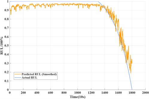
Table 3Comparison of TCN-GRU-SA, I-DCNN, CNN-Bi-LSTM, and TCN-GRU.
Bearing | I-DCNN | CNN-Bi-LSTM | TCN-GRU | TCN-GRU-SA | ||||
RMSE | MAE | RMSE | MAE | RMSE | MAE | RMSE | MAE | |
Bearing 1-3 | 0.2513 | 0.2190 | 0.1061 | 0.0818 | 0.1509 | 0.0831 | 0.0822 | 0.0582 |
Bearing 1-4 | 0.5236 | 0.4865 | 0.1916 | 0.1373 | 0.1210 | 0.0686 | 0.1032 | 0.0486 |
Bearing 1-5 | 0.2199 | 0.1949 | 0.2713 | 0.2198 | 0.0621 | 0.0570 | 0.0475 | 0.0319 |
Bearing 1-6 | 0.2002 | 0.1734 | 0.2115 | 0.1765 | 0.1044 | 0.0540 | 0.0730 | 0.0439 |
Bearing 1-7 | 0.2499 | 0.2145 | 0.1549 | 0.1180 | 0.0921 | 0.0634 | 0.1091 | 0.0801 |
4. Conclusions
This paper proposes a novel RUL prediction framework for rolling bearings that integrates adaptive signal decomposition with a parallel deep learning architecture. To address the limitations of fixed-parameter signal processing, a GWO-VMD algorithm is developed. By introducing a weighted kurtosis criterion, this method achieves adaptive parameter optimization, which significantly enhances the signal-to-noise ratio and allows for the effective extraction of degradation features from strong background noise.
Using the reconstructed signals, a parallel TCN-GRU-SA hybrid model is constructed to predict RUL. This architecture synergizes the strengths of dilated causal convolutions in capturing long-term dependencies and GRUs in modeling sequential dynamics. Furthermore, the integration of the Self-Attention mechanism enables the model to dynamically weight critical fault features while suppressing irrelevant interference. Experimental results on industrial bearing datasets demonstrate that the proposed framework achieves state-of-the-art performance in terms of RMSE and MAE, exhibiting superior robustness and prediction accuracy compared to traditional physics-based and single-model deep learning approaches.
However, several limitations remain to be addressed in future work. First, the determination of the degradation onset currently relies on expert-defined thresholds, which may introduce subjectivity; future studies will explore unsupervised change-point detection for adaptive thresholding. Second, the current experiments were conducted under constant operating conditions; extending the framework to multi-condition scenarios via domain adaptation or transfer learning is necessary. Finally, considering the computational complexity of the parallel architecture, future research will focus on lightweight model design (e.g., model pruning) and interpretability enhancement to facilitate real-time deployment in industrial edge computing systems.
References
-
J. Liu and Y. Shao, “Overview of dynamic modelling and analysis of rolling element bearings with localized and distributed faults,” Nonlinear Dynamics, Vol. 93, No. 4, pp. 1765–1798, May 2018, https://doi.org/10.1007/s11071-018-4314-y
-
C. Cheng et al., “A deep learning-based remaining useful life prediction approach for bearings,” IEEE/ASME Transactions on Mechatronics, Vol. 25, No. 3, pp. 1243–1254, Jun. 2020, https://doi.org/10.1109/tmech.2020.2971503
-
H. Wang, G. Ni, J. Chen, and J. Qu, “Research on rolling bearing state health monitoring and life prediction based on PCA and Internet of things with multi-sensor,” Measurement, Vol. 157, p. 107657, Jun. 2020, https://doi.org/10.1016/j.measurement.2020.107657
-
L. Guo, N. Li, F. Jia, Y. Lei, and J. Lin, “A recurrent neural network based health indicator for remaining useful life prediction of bearings,” Neurocomputing, Vol. 240, pp. 98–109, May 2017, https://doi.org/10.1016/j.neucom.2017.02.045
-
T. Li, H. Shi, X. Bai, and K. Zhang, “A fault diagnosis method based on stiffness evaluation model for full ceramic ball bearings containing subsurface cracks,” Engineering Failure Analysis, Vol. 148, p. 107213, Jun. 2023, https://doi.org/10.1016/j.engfailanal.2023.107213
-
F. König, J. Marheineke, G. Jacobs, C. Sous, M. J. Zuo, and Z. Tian, “Data-driven wear monitoring for sliding bearings using acoustic emission signals and long short-term memory neural networks,” Wear, Vol. 476, p. 203616, Jul. 2021, https://doi.org/10.1016/j.wear.2021.203616
-
H. Shi, M. Hou, Y. Wu, and B. Li, “Incipient fault detection of full ceramic ball bearing based on modified observer,” International Journal of Control, Automation and Systems, Vol. 20, No. 3, pp. 727–740, Mar. 2022, https://doi.org/10.1007/s12555-021-0167-0
-
Y. Lei, N. Li, S. Gontarz, J. Lin, S. Radkowski, and J. Dybala, “A model-based method for remaining useful life prediction of machinery,” IEEE Transactions on Reliability, Vol. 65, No. 3, pp. 1314–1326, Sep. 2016, https://doi.org/10.1109/tr.2016.2570568
-
Y. Zhang, J. Sun, J. Zhang, H. Shen, Y. She, and Y. Chang, “Health state assessment of bearing with feature enhancement and prediction error compensation strategy,” Mechanical Systems and Signal Processing, Vol. 182, p. 109573, Jan. 2023, https://doi.org/10.1016/j.ymssp.2022.109573
-
B. Li, B. Tang, L. Deng, and M. Zhao, “Self-attention ConvLSTM and its application in RUL prediction of rolling bearings,” IEEE Transactions on Instrumentation and Measurement, Vol. 70, pp. 1–11, Jan. 2021, https://doi.org/10.1109/tim.2021.3086906
-
L. Song, T. Lin, Y. Jin, S. Zhao, Y. Li, and H. Wang, “Advancements in bearing remaining useful life prediction methods: a comprehensive review,” Measurement Science and Technology, Vol. 35, No. 9, p. 092003, Sep. 2024, https://doi.org/10.1088/1361-6501/ad5223
-
J. Zhou, J. Yang, Q. Qian, and Y. Qin, “A comprehensive survey of machine remaining useful life prediction approaches based on pattern recognition: taxonomy and challenges,” Measurement Science and Technology, Vol. 35, No. 6, p. 062001, Jun. 2024, https://doi.org/10.1088/1361-6501/ad2bcc
-
B. Yang, R. Liu, and E. Zio, “Remaining useful life prediction based on a double-convolutional neural network architecture,” IEEE Transactions on Industrial Electronics, Vol. 66, No. 12, pp. 9521–9530, Dec. 2019, https://doi.org/10.1109/tie.2019.2924605
-
H. Ding, L. Yang, Z. Cheng, and Z. Yang, “A remaining useful life prediction method for bearing based on deep neural networks,” Measurement, Vol. 172, p. 108878, Feb. 2021, https://doi.org/10.1016/j.measurement.2020.108878
-
J. Luo and X. Zhang, “Convolutional neural network based on attention mechanism and Bi-LSTM for bearing remaining life prediction,” Applied Intelligence, Vol. 52, No. 1, pp. 1076–1091, May 2021, https://doi.org/10.1007/s10489-021-02503-2
-
S. Liu, M. Liu, Y. He, H. Han, and Y. Meng, “Bearing remaining useful life prediction based on DCNN network and self-attention-BiGRU mechanism,” (in Chinese), Journal of Mechanical and Electrical Engineering, Vol. 41, pp. 786–796, 2024, https://doi.org/10.3969/j.issn.1001-4551.2024.05.004
-
W. Cao, Z. Meng, J. Li, J. Wu, and F. Fan, “A remaining useful life prediction method for rolling bearing based on TCN-transformer,” IEEE Transactions on Instrumentation and Measurement, Vol. 74, pp. 1–9, Jan. 2025, https://doi.org/10.1109/tim.2024.3502878
-
K. Dragomiretskiy and D. Zosso, “Variational mode decomposition,” IEEE Transactions on Signal Processing, Vol. 62, No. 3, pp. 531–544, Feb. 2014, https://doi.org/10.1109/tsp.2013.2288675
-
S. Mirjalili, S. M. Mirjalili, and A. Lewis, “Grey Wolf optimizer,” Advances in Engineering Software, Vol. 69, pp. 46–61, Mar. 2014, https://doi.org/10.1016/j.advengsoft.2013.12.007
-
S. Zhang, X. Wang, X. Li, and C. Yang, “Fault feature extraction method for rolling bearings based on FVMD,” (in Chinese), Journal of Vibration and Shock, Vol. 41, pp. 236–244, 2022, https://doi.org/10.13465/j.cnki.jvs.2022.06.030
-
S. Bai, J. Z. Kolter, and V. Koltun, “An empirical evaluation of generic convolutional and recurrent networks for sequence modeling,” arXiv:1803.01271, Jan. 2018, https://doi.org/10.48550/arxiv.1803.01271
-
K. Cho et al., “Learning phrase representations using RNN encoder-decoder for statistical machine translation,” arXiv:1406.1078, Jan. 2014, https://doi.org/10.48550/arxiv.1406.1078
-
Y. Xiao, C. Zou, H. Chi, and R. Fang, “Boosted GRU model for short-term forecasting of wind power with feature-weighted principal component analysis,” in Energy, Vol. 267, p. 126503, Mar. 2023, https://doi.org/10.1016/j.energy.2022.126503
-
P. Nectoux et al., “An experimental platform for bearings accelerated degradation tests,” in IEEE International Conference on Prognostics and Health Management, Jun. 2012.
-
Y. Guo et al., “An improved deep convolution neural network for predicting the remaining useful life of rolling bearings,” Journal of Intelligent and Fuzzy Systems, Vol. 40, No. 3, pp. 5743–5751, Mar. 2021, https://doi.org/10.3233/jifs-201965
-
F. Li, Z. Dai, L. Jiang, C. Song, C. Zhong, and Y. Chen, “Prediction of the remaining useful life of bearings through CNN-Bi-LSTM-based domain adaptation model,” Sensors, Vol. 24, No. 21, p. 6906, Oct. 2024, https://doi.org/10.3390/s24216906
About this article

This research was funded by the National Natural Science Foundation of China, grant numbers 61773225, and the Zhejiang Natural Science Foundation, grant number LY20A010012.
The datasets generated during and/or analyzed during the current study are available from the corresponding author on reasonable request.
Lingbin Kong: formal analysis, writing-original draft preparation. Yang Chen: conceptualization, methodology, writing-review and editing. Xiaoyan Mao: supervision, funding acquisition. Yongqi Chen: supervision, writing-review and editing. Zongcai Ma: formal analysis, validation.
The authors declare that they have no conflict of interest.
