Effect of parametric modulation on the stability of a periodic oscillator: a study with Airy functions

1. Introduction

In recent years, systems with variable stiffness have attracted attention in control engineering. These systems exploit the modulation of stiffness properties to achieve objectives such as vibration attenuation and resonance suppression to improve structural performance. The stiffness variation is typically implemented via a control law that switches between two discrete values, allowing the system to adapt its response to operational conditions or external disturbances [1-6].

Among the contributions in this area, Moreno and Diarte [1] propose a control law in which the switching is state-dependent. Their work demonstrates that such a strategy effectively mitigates mechanical vibrations in linear time-invariant (LTI) systems. The underlying principle is that by appropriately alternating the stiffness, one can induce energy dissipation. Nevertheless, the introduction of a switching control law also introduces significant analytical challenges. Specifically, the system becomes inherently time-varying, departing from the standard analysis of LTI systems. In general, time-varying systems – particularly those with discontinuous coefficients – are difficult to analyze, as classical tools such as eigenvalue analysis and transfer functions are no longer directly applicable. The example analyzed by Moreno and Diarte is the Reid oscillator, written as follows:

where the stiffness function is defined as $\stackrel{-}{k}\left(t\right)=1+\epsilon sgn\left(x\dot{x}\right)$, with $sgn(\bullet )$ denoting the sign function and $0<\epsilon <1$ a real constant. The non-dimensional adjustment parameter $\epsilon$ plays a pivotal role in governing the dynamics of the system, determining the rate at which oscillations are attenuated. In addition, this parameter has served as a standard metric for assessing the performance of semi-active stiffness devices [6].

To analyze the system, we must note that it has a non-continuous coefficient $\stackrel{-}{k}\left(t\right)$. Consequently, the use of specialized mathematical tools for time-varying systems is required. Such tools often involve sophisticated techniques, including numerical simulations, piecewise analysis, or perturbation methods. These tools are generally not easy to use. Remarkably, in this case, $\stackrel{-}{k}\left(t\right)$ exhibits periodic behavior. This periodicity allows for the application of Floquet theory, a rigorous framework for studying the stability and qualitative behavior of linear systems with periodic coefficients, thereby classifying the Reid oscillator as a Hill-type system [7, 8].

Although Floquet theory is generally considered mathematically demanding, the alternating nature of $\stackrel{-}{k}\left(t\right)$ between two constant values (commutation) simplifies the analysis. This property enables the derivation of analytical solutions, similar in approach to the classical Meissner equation [9]. These analytical expressions not only enhance theoretical understanding but also provide benchmarks for validating numerical simulations and experimental investigations.

Until now, the study of variable-stiffness systems has been only partially addressed: most research has focused on the restrictive scenario in which stiffness alternates instantaneously between two constants. While this assumption renders the problem mathematically tractable, it does not fully capture the complexity of real-world applications, where switching may be non-instantaneous or involve more complex stiffness profiles. Therefore, bridging the gap between idealized commutated models and practically implementable controllers remains an open problem.

In this work, we address this gap by studying a variant derived from the commutation-based control law proposed in [2], in which stiffness transitions occur over a finite switching interval. This alteration fundamentally changes the problem: the switching instants can no longer be determined analytically in advance, and the system coefficient is no longer piecewise constant. As a result, the analytical tools traditionally used for the classical Reid and Hill oscillators are no longer directly applicable. A key contribution of this work is the derivation of explicit analytical solutions in terms of Airy functions. These solutions do not merely reproduce known Floquet stability patterns; rather, they reveal how the finite transition duration reshapes the boundaries between stability and instability and quantifies the corresponding rate of energy dissipation. To the best of our knowledge, no prior study has established this analytical connection between smooth stiffness transitions, Airy-function solutions, and vibration-attenuation performance.

2. Problem statement

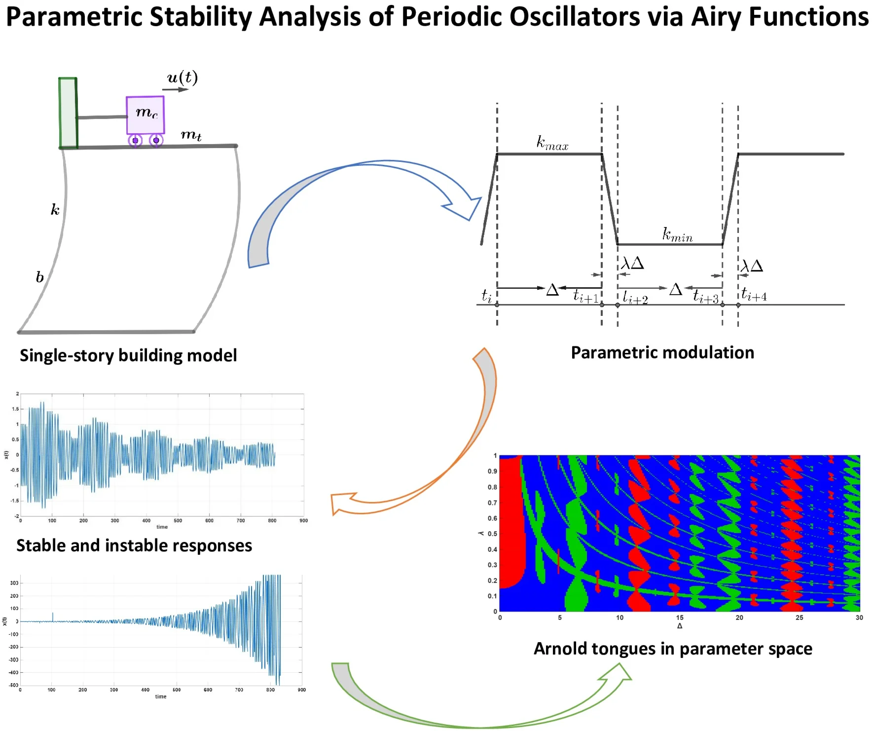
In [3], a state-dependent controller was designed and experimentally implemented to mitigate mechanical vibrations induced by seismic excitations. The control strategy was applied to a single-story building model, schematically represented in Fig. 1, where a movable mass $m_c$ traverses a linear path. The motion of this mass is designed to attenuate the vibrations experienced by the building structure during a seismic event.

The mathematical model can be expressed as:

where $m=m_c+m_t$, $m_c$ is a linearly moving mass and $m_t$ is the mass of the building roof. The coefficient $b$ accounts for viscous damping associated with the walls, while $k$ denotes the structural stiffness of the building. For more details of the model see [10].

Let us consider a control input of the form $u=-\widehat{k}\left(t\right)x\left(t\right)$ and assume that $b\ll 1$. Substituting this control law into the Eq. (2) yields:

where $k\left(t\right)=(k+\widehat{k}\left(t\right))/m$, is the time-dependent equivalent stiffness of the building-mass system, with units [N/m]. As we can see, this model corresponds to the form of Eq. (1). By appropriate manipulation of the model, we identify $k\left(t\right) = \stackrel{-}{k}\left(t\right)$ expecting to reproduce the same behavior reported in [1]. However, the experimental results show discrepancy in the controller response. The switching is not instantaneous, contrary to the idealized assumption. The motion of the mass $m_c$ remains subject to the physical constraints of the experiment, which inherently introduce short transition intervals between the stiffness states. This phenomenon is illustrated in Fig. 2, the switching between the minimum and maximum values of $k\left(t\right)$ occurs over a finite duration rather than abruptly. This duration is relatively short, but this time can increase whether the experimental conditions change, for instance, if the mass $m_c$ has to increase its travel or a higher friction.

Fig. 1Single-story building model

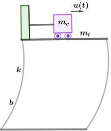
Fig. 2Experimental data of k(t)

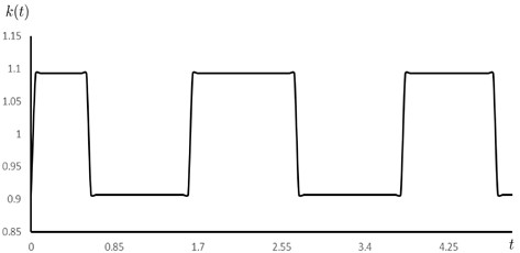
These observations motivate an analysis of the system in which the stiffness switching is non-instantaneous. We propose the model depicted in Fig. 3, where the stiffness function $k\left(t\right)$ alternates periodically between two values $k_{max}$ and $k_{min}$, but with finite rising and falling transitions. These rises and falls are assumed to be linear in a small-time interval. The resulting model no longer corresponds to a purely piecewise-constant system, but rather to a continuous, piecewise-linear periodic system. Therefore, the central problem addressed in this work is the characterization and analysis of a linear oscillator with non-instantaneous, linearly varying stiffness switching.

3. Preliminaries

Let us consider Eq. (3). The solutions of Eq. (3) depend directly on the stiffness function $k\left(t\right)$. Two representative cases are distinguished below.

3.1. Case 1. Constant stiffness

If $k\left(t\right)$ is any value $k_{max}$, $k_{min}>0$, the Eq. (3) reduces to the classical linear oscillator equation:

4

$\ddot{x}\left(t\right)+kx\left(t\right)=0,\mathrm{ }\mathrm{ }x\left(t_0\right)=x_0,\mathrm{ }\mathrm{ }\dot{x}\left(t_0\right)={\dot{x}}_0.$

Fig. 3Non-instantaneous switching of k(t)

The solution is well known and can be expressed as:

$\left(\begin{array}{c}x\left(t\right)\\ \dot{x}\left(t\right)\end{array}\right)=\left(\begin{array}{cc}\cos \left(\sqrt{k}(t-t_0)\right)& \frac{1}{\sqrt{k}}\sin \left(\sqrt{k}(t-t_0)\right)\\ -\sqrt{k}\sin \left(\sqrt{k}(t-t_0)\right)& \cos \left(\sqrt{k}(t-t_0)\right)\end{array}\right)\left(\begin{array}{c}{x}_0\\ {\dot{x}}_0\end{array}\right),$

while the transition matrix is given by:

$\mathrm{\Phi }\left({\mathrm{t}}_0,t_1\right)=\left(\begin{array}{cc}\cos \left(\sqrt{k_{max}}(t_1-t_0)\right)& \frac{1}{\sqrt{k_{max}}}\sin \left(\sqrt{k_{max}}(t_1-t_0)\right)\\ -\sqrt{k_{\mathit{max}}}\sin \left(\sqrt{k_{max}}(t_1-t_0)\right)& \cos \left(\sqrt{k_{max}}(t_1-t_0)\right)\end{array}\right).$

4. Results

We assume that the function $k\left(t\right)$ is periodic and defined as follows (see Fig. 3):

where $m=\frac{\left(k_{max}-k_{min}\right)}{\lambda \mathrm{\Delta }}$, for $i=\mathrm{0,1},2,\dots$ and a small parameter $\lambda \in \left(\mathrm{0,1}\right).$

Once defined $k\left(t\right)$, we can obtain the corresponding transition matrix for each interval as follows.

Interval $[t_0,t_1)$. In this case $k\left(t\right)=k_1\left(t\right)=k_{max}$ and Eq. (3) reduces to $\ddot{x}\left(t\right)+k_1\left(t\right)x\left(t\right)=0$, $x\left(t_0\right)=x_0$, $\dot{x}\left(t_0\right)={\dot{x}}_0.$ The transition matrix from $t_0$ to $t_0+\mathrm{\Delta }=t_1$ is:

and we have $\left(\begin{array}{c}{x}_1\\ {\dot{x}}_1\end{array}\right)={\mathrm{\Phi }}_1\left(t_0,t_1\right)\left(\begin{array}{c}{x}_0\\ {\dot{x}}_0\end{array}\right).$

– Interval $[t_1,t_2)$. Here $k\left(t\right)=k_2\left(t\right)=-mt+m\left[i\right(1+\lambda )+1]∆+k_{max}$. Then Eq. (3) becomes $\ddot{x}\left(t\right)+k_2\left(t\right)x\left(t\right)=0$, $x\left(t_1\right)=x_1$, $\dot{x}\left(t_1\right)={\dot{x}}_1.$

The corresponding fundamental matrix is:

where $\tau \left(t\right)={-k}_2\left(t\right)/m^{2/3}$.

The transition matrix is from $t_1$ to $t_2=t_1+\lambda \mathrm{\Delta }$ is ${\mathrm{\Phi }}_2\left(t_1,t_2\right)={\mathrm{\Psi }}_1\left(t_2\right){\mathrm{\Psi }}_1^{-1}\left(t_1\right)$ and $\left(\begin{array}{c}{x}_2\\ {\dot{x}}_2\end{array}\right)={\mathrm{\Phi }}_2\left(t_1,t_2\right)\left(\begin{array}{c}{x}_1\\ {\dot{x}}_1\end{array}\right).$

– Interval $[t_2,t_3)$. For $k\left(t\right)=k_3\left(t\right)=k_{min}$, we have $\ddot{x}\left(t\right)+k_3\left(t\right)x\left(t\right)=0$, $x\left(t_2\right)=x_2$, $\dot{x}\left(t_2\right)={\dot{x}}_2.$ The transition matrix in the interval is:

and $\left(\begin{array}{c}{x}_3\\ {\dot{x}}_3\end{array}\right)={\mathrm{\Phi }}_3\left(t_2,t_3\right)\left(\begin{array}{c}{x}_2\\ {\dot{x}}_2\end{array}\right)$.

– Interval $[t_3,t_4)$. Finally, $k\left(t\right)=k_4\left(t\right)=mt-m\left[\right(i+1\left)\right(1+\lambda )+1]∆+k_{min}$. The fundamental matrix is:

where $\tau \left(t\right)={-k}_4\left(t\right)/m^{2/3}$. Then ${\mathrm{\Phi }}_4\left(t_4,t_3\right)={\mathrm{\Psi }}_2\left(t_4\right){\mathrm{\Psi }}_2^{-1}\left(t_3\right)$.

Using the Airy Wronskian identity $W(Ai,Bi)=1/\pi$, it follows that $\det \left({\mathrm{\Psi }}_1\left(t\right)\right)=\det \left({\mathrm{\Psi }}_2\left(t\right)\right)=\frac{m^{1/3}}{\pi }$, which is constant in time. This constant determinant is explicitly taken into account when computing ${\mathrm{\Psi }}_1^{-1}\left(t_1\right)$ and ${\mathrm{\Psi }}_2^{-1}\left(t_3\right)$, ensuring correct normalization in the construction of the transition matrix.

Due to the periodicity of $k\left(t\right)$, the procedure can be repeated identically for any number of periods $T=2(1+\lambda )\mathrm{\Delta }$. Consequently, $\left(\begin{array}{c}x\left(T\right)\\ \dot{x}\left(T\right)\end{array}\right)={{{\mathrm{\Phi }}_4\left(t_4,t_3\right)\mathrm{\Phi }}_3\left(t_3,t_2\right){\mathrm{\Phi }}_2\left(t_1,t_2\right)\mathrm{\Phi }}_1\left(t_0,t_1\right)\left(\begin{array}{c}{x}_0\\ {\dot{x}}_0\end{array}\right).$

Defining the matrix:

known as the monodromy matrix, the evolution after $n$ periods satisfies:

The eigenvalues of $\mathrm{\Phi }\left(T\right)$, denoted by $\rho$ are the Floquet multipliers, which determine the stability of the system. The stability criterion is as follows: If $\left|\rho \right|<1$ for all Floquet multipliers, then the solution is asymptotically stable. Unstable solutions are classified according to the nature of the dominant Floquet multiplier. A positive real multiplier (${\rho }_{max} >1)$ indicates a period-𝑇 instability; a negative real multiplier (${\rho }_{max} <-1)$ corresponds to a period-2𝑇 instability; and a complex conjugate pair with amplitude larger than one $\left|{\rho }_{max} \right|>1$ indicates a parametric resonance characterized by oscillatory, multi-periodic growth.

This classification is used throughout the numerical analysis presented in Figs. 4-6. The time-domain responses in Figs. 4 and 5 were obtained via numerical integration using a Runge-Kutta 4(5) adaptive scheme, whereas the stability chart in Fig. 6 was computed by evaluating the spectral radius of the monodromy matrix associated with one full switching period. All simulations and calculations were conducted in MATLAB R2025b. The numerical results correspond to the parameter sets listed in Table 1. Note that the system response can be either stable or unstable depending on the selected parameters: for the stable case, the maximum Floquet multiplier is $\left|{\rho }_{max}\right|=\text{0.9211}$, whereas for the unstable case $\left|{\rho }_{max}\right|=\text{1.3402}$.

Fig. 4Stable numerical solution x(t) when Δ=20 and λ=0.01

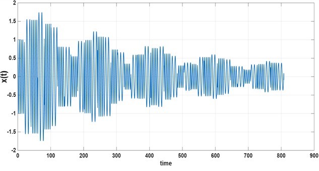
Fig. 5Unstable numerical solution x(t) when Δ= 20 and λ=0.04

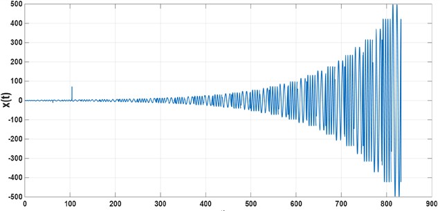
At first glance, it might appear that increasing the value of $\lambda$ lead to a unstable solution, since changing $\lambda$ from 0.01 to 0.04 results in a transition from stable to unstable behavior. However, this trend does not hold globally in the parameter space: when we change $\mathrm{\Delta }$ from 20 to 10 keeping $\lambda$ = 0.04, the solution becomes stable again, with $\left|{\rho }_{max}\right|=\text{0.6962.}$ Fig. 6 presents a 3D map of the maximum Floquet multiplier as a function of the parameters $(\mathrm{\Delta },\lambda )$. The contour plot included in the same figure highlights the stability boundary defined by $\left|{\rho }_{max}\right|=1$. Regions below this contour correspond to asymptotically stable solutions, while regions above it correspond to instability.

As illustrated in Fig. 7, the parameter plane exhibits a structured organization of dynamical responses. A large stable region (blue) is separated from a domain of period-T instability (red), while the emergence of parametric resonance (green) forms well-defined resonance tongues. This demonstrates that even small variations of the parameters may lead to a sudden transition from stable motion to strongly amplified oscillations.

Fig. 6Dependence of |ρmax | on the parameters Δ and λ

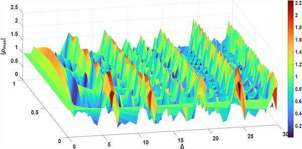
a) 3D map of $\left|{\rho }_{max}\right|$

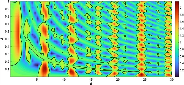
b) Contour map: $\left|{\rho }_{max}\right|=1$

Fig. 7Instability classification: blue – stable; red – Period-T instability; green – parametric resonance

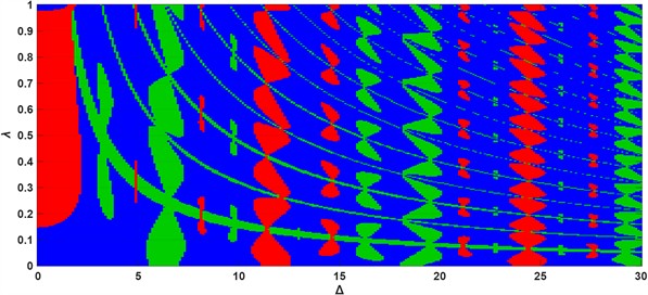
The stability transitions observed in the $(\mathrm{\Delta },\lambda )$-plane have direct relevance for real vibration-control systems in which the stiffness is periodically modulated, either intentionally (e.g., parametric controllers) or unintentionally (e.g., structural degradation or load fluctuations). In this context, the appearance of alternating regions of stability and instability provides a practical guideline for controller design: increasing the modulation amplitude $\lambda$ does not necessarily destabilize the system, and the effect critically depends on the $(\mathrm{\Delta },\lambda )$ parameters interaction.

The parameter $\lambda$ does not merely represent a small perturbation of the excitation profile; rather, it controls the spectral content of the parametric modulation $k\left(t\right)$. When $\lambda =0$, the piecewise-constant excitation has a Fourier series rich in harmonics. Increasing $\lambda$ introduces a linear ramp that effectively acts as a low-pass filter, attenuating the higher-order harmonics of the excitation.

Overall, the results highlight that effective parametric control requires not only tuning the amplitude of stiffness variation but also its timing. The Floquet multipliers provide a quantitative indicator for selecting safe operating regions and preventing undesired transitions to exponentially growing oscillations.

Finally, a closed-form analytical approximation of the transition matrices may be derived by replacing the Airy functions by their asymptotic expansions for large positive and negative arguments. Such an approach would lead to perturbative expressions for the monodromy matrix, potentially yielding an approximate analytical stability condition similar to the Whittaker-Ince-Straus relation in the Mathieu case. However, the present study explores parameter regimes where the arguments of the Airy functions are not asymptotically large, and therefore we evaluate ${\mathrm{\Phi }}_2$ and ${\mathrm{\Phi }}_4$ numerically to ensure uniform accuracy in the entire stability map.

5. Conclusions

The analysis of Floquet multipliers as a function of the parameters $\mathrm{\Delta }$ and $\lambda$ shows a structure of alternating bands of stability and instability (Arnold tongues), characteristic of Hill-type systems. As $\mathrm{\Delta }$ increases, recurrent regions of parametric resonance are observed, where small variations in periodicity cause transitions between stable and exponentially growing solutions. On the other hand, the parameter $\lambda$ regulates the extension of the temporal variation of $k\left(t\right)$; small values produce stable, quasi-harmonic behavior, while large values introduce instabilities by increasing the influence of the linear temporal variation regions. In these intervals, the solutions are expressed by Airy functions, the combination of which determines whether the response is attenuated or amplified between periods. Overall, the results show that the stability of the system depends on the balance between the periodicity imposed by $\mathrm{\Delta }$ and the parametric modulation controlled by $\lambda$, mediated by the transitional dynamics represented by the Airy functions.

Although the complete formulation of the unforced mechanical system possesses an underlying Hamiltonian structure, the approximation $b\ll 1$ used in this study does not explicitly preserve that property. Nevertheless, this reduction isolates the dominant mechanism responsible for stability loss, and the Floquet spectrum obtained numerically shows that any departure from exact Hamiltonian symmetry is of higher order and does not alter the onset or nature of the observed instabilities.

We acknowledge that the prescribed piecewise-linear profile for $k\left(t\right)$ constitutes an idealized representation of actuator-driven stiffness modulation. This formulation was adopted because it enables an analytically tractable characterization of the transition matrices and the resulting monodromy matrix, allowing us to isolate and study the specific effect of finite transition time on stability. While more realistic actuator-coupled models may introduce additional dynamical effects that are outside the scope of the present work, we expect the qualitative trends reported here to remain relevant. Extending the analysis to more general transition laws represents a natural continuation of this line of research.