Sensor placement method for crane structural health monitoring based on multi-level damage identification

Liu, Guansi; Jin, Hui; Ding, Keqin

doi:10.21595/jve.2026.25812

Journal of Vibroengineering

Browse Journal

Submit article

Published: May 16, 2026

Check for updates

Sensor placement method for crane structural health monitoring based on multi-level damage identification

Guansi Liu¹

Hui Jin²

Keqin Ding³

^{1, 2}Jiangsu Key Laboratory of Engineering Mechanics, School of Civil Engineering, Southeast University, Nanjing, 211189, China

³China Special Equipment Inspection and Research Institute, Beijing, 100029, China

Corresponding Author:

Hui Jin

Cite the article Download PDF

Article in Press

Downloads 17

Abstract

Local damages such as microcracks and corrosion in crane steel structures often exhibit strong localization and weak mode shape perturbation characteristics. Especially when the damage scale is smaller than the modal wavelength, it cannot be simply treated as an overall damage issue for identification. In response to the diverse damage modes of crane structures and the need for dense sensor placement for local identification, a sensor optimization placement method based on multi-level damage feature fusion is proposed. Firstly, structural sub-regions are divided according to the main beam diaphragms, and sensors are arranged with boundary points as key measurement points. The displacement frequency response amplitude changes before and after damage are utilized to identify damage and eliminate insensitive measurement points to complete preliminary optimization. Secondly, a displacement frequency response amplitude change matrix is constructed, and the damage signal is enhanced through cross-frequency weighted superposition to form a damage identification vector, accurately locating the damage occurrence area. Furthermore, node-level correction is performed in candidate areas based on displacement flexibility difference values, and precise localization of damage points is achieved through priority sorting of flexibility differences. Simulation results show that under the condition where corrosion damage is set in units 20739, 20762, and 20785, the maximum point of the flexibility difference damage index is located in unit 20762, which coincides with the preset damage location, verifying the effectiveness of the hierarchical placement strategy from initial damage screening to precise localization.

1. Introduction

Cranes are core equipment in industrial fields such as metallurgy and ports. The increasing complexity of their structures and the integration of functions have made structural health monitoring systems crucial for ensuring their safe operation. The optimal placement of sensors is the primary step in the monitoring system, directly determining the effectiveness of capturing damage characteristics. However, in practical engineering, the number of sensors is often severely limited. How to achieve accurate identification and localization of complex structural damage with limited measurement points is a pressing issue that needs to be addressed. Focusing on this challenge, research at home and abroad mainly unfolds from two dimensions: damage identification methods and sensor optimization placement. Wu, Duo, et al. [1] proposed an optimization algorithm based on the Modal Assurance Criterion, which iteratively increases and decreases the number of sensors to address the deficiency of traditional methods that overly rely on the initial selection of measurement points. Its engineering applicability was verified through a numerical example and a real bridge. Shuigen Hu et al. [2] proposed a method combining progressive continuous wavelet transform and singular value decomposition. This method addresses the insensitivity of mode shapes to local damage and the sensitivity of modal curvature by denoising and enhancing damage features to identify structural damage from noisy mode shapes. Cao Maosen et al. [3] proposed a two-step damage localization strategy for beam structures. This strategy first uses the change in natural frequency to preliminarily determine the approximate damage region, and then employs the modal shape curvature to accurately identify the specific damage location. According to the physical parameters utilized, existing damage identification methods can be summarized into the following categories: First, methods based on modal parameters, which utilize changes in parameters such as frequency, mode shape, and curvature mode for identification and localization [4-6]; second, methods based on flexibility matrices, which are sensitive to local stiffness changes and achieve damage detection by constructing or comparing flexibility matrices and their derived indicators (such as modal curvature and flexibility difference) [7-11]; third, methods based on parameter identification and statistical inference, aimed at enhancing robustness in noisy environments, such as combining Kalman filtering, frequency response functions, and probabilistic statistical methods [12-16]. In terms of sensor optimization placement, research focuses on maximizing information acquisition under given measurement point constraints through eigenvector sensitivity, dual sensitivity analysis, or multi-objective intelligent optimization algorithms [17, 18]. In addition to the above classical research threads, multi-source information fusion and intelligent algorithms are becoming new trends. For example, strategies combining model reduction and response reconstruction aim to achieve global response estimation with a small number of sensors, thereby supporting damage identification [19]; global damage identification methods based on multi-source signals (such as vibration and strain) and spatiotemporal graph neural networks (ST-GNN) frameworks attempt to mine deep damage characteristics through data-driven models [20]. Additionally, there are integrated approaches combining strain sensing, artificial intelligence, and meta-heuristic optimization algorithms [21]. These emerging methods show potential in enhancing the representation ability and automation level of complex damage patterns.

However, despite the progress made by existing methods under their respective specific conditions, most of them still generally face common issues such as dependence on prior models or dense measurement points, as well as decreased identification accuracy and reliability in early micro-damage and multi-damage scenarios. Therefore, how to comprehensively utilize multi-source damage features to construct a progressive identification system from damage screening to precise localization has become the key to enhancing the practicality of monitoring systems. This paper aims to study the optimal sensor placement method based on multi-level damage features, achieving efficient and accurate damage identification under limited sensor conditions by integrating different levels of sensitive indicators, providing a new solution for the safe operation and maintenance of important structures such as cranes.

2. Sensor placement method for multi-level progressive damage identification

Structural damage detection based on modal frequencies is regarded as an inverse eigenvalue problem. A free vibration eigenvalue problem of a discrete system with $n$ degrees of freedom is described by the following equation:

1

(K - ω^{2} M) Φ = 0 .

Among them, $ω$ is the order eigenvalue (square of natural frequency), and $Φ$ is the corresponding eigenvector (mode shape), $Φ = [ϕ_{1}, ϕ_{2}, ϕ_{3}, \dots ϕ_{n}]$ .

The equation has $n$ solutions of eigenvalues and eigenvectors. These $n$ uncorrelated basis vectors can be normalized to obtain $n$ orthogonal vectors, namely the main mode $ϕ_{i}$ of each order. Arrange $ϕ_{i}$ into an $n \times n$ matrix, which is the mode matrix [1, 2]:

2

(K - {ω_{i}}^{2} M) ϕ_{i} = 0 .

The above analysis shows that:

3

\{\begin{matrix} {ϕ_{j}}^{T} (K - {ω_{i}}^{2} M) ϕ_{i} = 0, \\ {ϕ_{j}}^{T} (K - {ω_{j}}^{2} M) ϕ_{i} = 0 . \end{matrix}

From Eq. (3), it can be further obtained that:

4

({ω_{i}}^{2} - {ω_{j}}^{2}) {ϕ_{j}}^{T} M ϕ_{i} = \{\begin{matrix} {ϕ_{j}}^{T} M ϕ_{i} = 0, i \neq j, \\ {ϕ_{j}}^{T} M ϕ_{i} = m_{i}, i = j, \end{matrix}

5

{ϕ_{j}}^{T} (K - {ω_{i}}^{2} M) ϕ_{i} = \{\begin{matrix} {ϕ_{j}}^{T} M ϕ_{i} = 0, i \neq j, \\ {ϕ_{i}}^{T} K ϕ_{i} - {ω_{i}}^{2} m_{i} = 0, i = j, \end{matrix}

where, ${ϕ_{j}}^{T} M ϕ_{i} = m_{i}$ , then $Φ^{T} M Φ = d i a g [m_{i}]$ is the definition of modal mass, ${ϕ_{i}}^{T} K ϕ_{i} = k_{i}$ , then $Φ^{T} K Φ = d i a g [k_{i}]$ is the definition of stiffness mode.

Eq. (6) can be written as $K Φ = M Φ Λ$ , $Λ = d i a g [ω_{i}^{2}]$ and both sides can be right multiplied by $Φ^{T} M Φ$ :

6

K Φ Φ^{T} M Φ = M Φ Λ Φ^{T} M Φ .

Further multiply $(d i a g [m_{i}])^{- 1} Φ^{- 1}$ on the right-hand side of Eq. (6) to obtain the stiffness matrix of the structure:

7

K = M Φ Λ Φ^{T} M Φ (d i a g [m_{i}])^{- 1} Φ^{- 1} = \sum_{i = 1}^{n} \frac{{ω_{i}}^{2}}{m_{i}} M ϕ_{i} {ϕ_{i}}^{T} M .

Since $Φ^{T} K Φ = d i a g [k_{i}]$ , the inverse of both sides can be obtained simultaneously:

8

Φ^{- 1} K^{- 1} Φ^{- T} = (d i a g [m_{i}])^{- 1} (d i a g [{ω_{i}}^{2}])^{- 1}

By simultaneously multiplying $Φ$ and $Φ^{T}$ on both ends of Eq. (8), the structural flexibility matrix represented by modal parameters can be obtained:

9

F_{d} = K^{- 1} = Φ (d i a g [m_{i}])^{- 1} (d i a g [λ_{i}])^{- 1} Φ^{T} = \sum_{i = 1}^{n} \frac{1}{m_{i} {ω_{i}}^{2}} ϕ_{i} ϕ_{i}^{T} .

The flexibility matrix $F_{d}$ is inversely proportional to the square of the natural frequency, so the accurate flexibility matrix can be obtained only by obtaining the low-order modal information of the structure. By quantifying the deformation characteristics and modal response of the structure under load, the flexibility matrix can accurately guide the optimal placement of sensors.

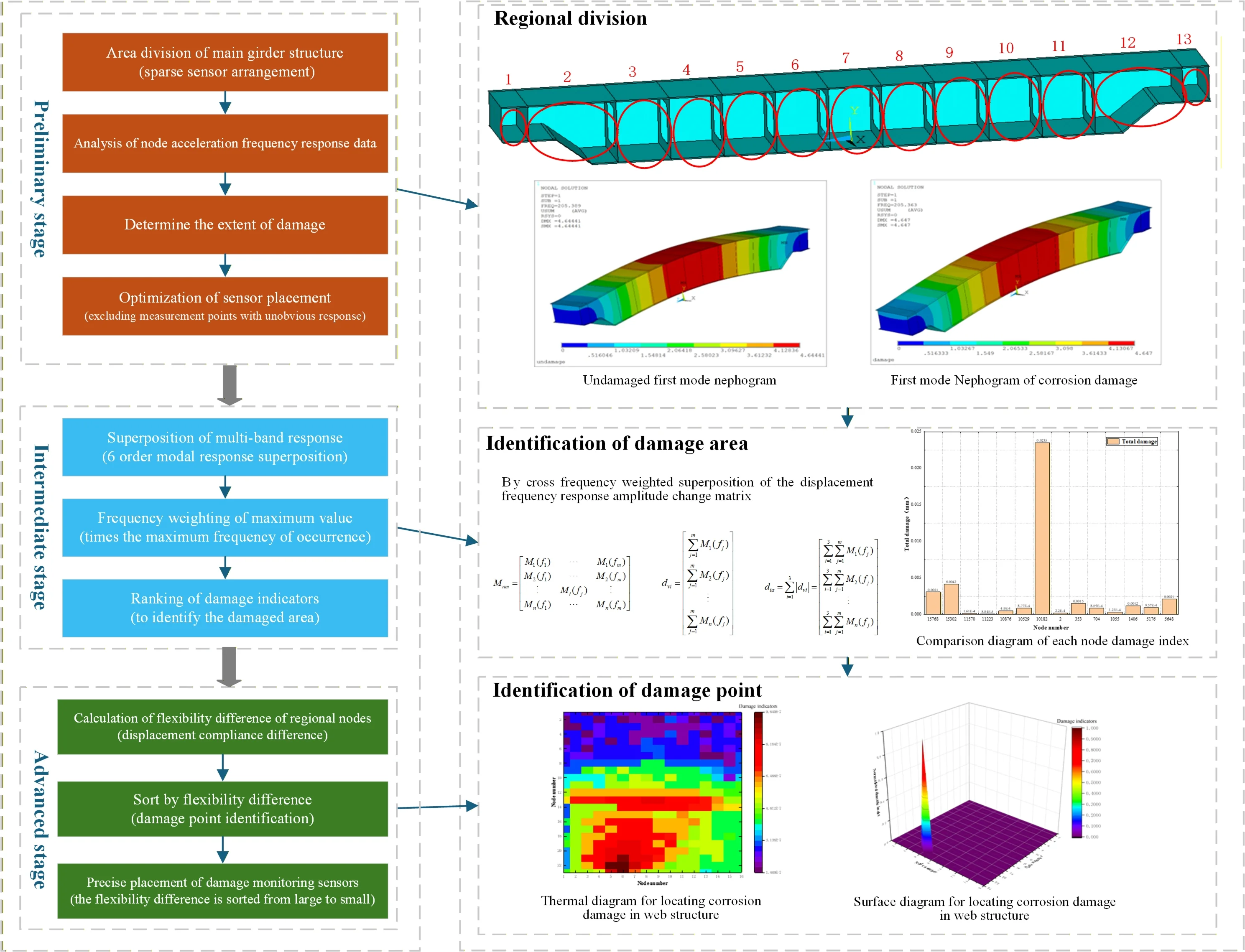
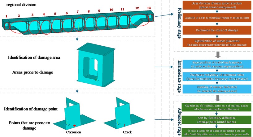
In order to effectively monitor complex structures, a hierarchical approach is often adopted to determine the existence and location of damage in a stepwise manner. The optimal sensor placement can be achieved through three stages: initial (layout of boundary points to determine whether damage exists) → intermediate (response enhancement of measurement points to identify the damage region) → advanced (precise sensor placement to locate the specific damage). This multi-level damage identification sensor placement method provides a theoretical basis and operational pathway for rationally guiding sensor deployment by progressively refining and enhancing damage identification capability. The sensor placement method for multi-level damage identification is illustrated in Fig. 1.

2.1. Initial stage: sensor placement based on region division

Based on the geometric characteristics of the structure, the overall structure is divided into several sub-regions with the main beam diaphragm as the boundary. The boundary points at the intersection of the diaphragm and the web plate are discontinuous in structural geometry and stiffness, forming a key path for internal force transfer in a dynamic sense and exhibiting high sensitivity to local stiffness changes. Changes in dynamic responses (such as acceleration frequency response functions) at these locations can reveal abnormal states of the overall structure earlier and more significantly. Therefore, sensors can be arranged at the boundary points as initial measuring points to obtain acceleration signals at the boundaries of each sub-region.

Fig. 1Sensor placement method for multi-level damage identification

The time-domain acceleration response of the structure under sinusoidal excitation is transformed into the frequency-domain response, and the damage location is further identified by using the frequency response amplitude change of the displacement response of the structure at the same position before and after the damage. $D_{i} (f_{j})$ is defined as the amplitude variation of displacement frequency response before and after damage:

10

D_{i} (f_{j}) = d_{i} (f_{j})^{u} - d_{i} (f_{j})^{d},

where $d_{i} (f_{j})$ is the displacement amplitude of node $i$ corresponding to frequency $f_{j}$ , $j$ is the node number corresponding to displacement output, $i =$ 1, 2,..., $n$ , subscript $j$ is the output band number, $j =$ 1,2,..., $m$ , superscripts $u$ and $d$ denote the intact and damaged states of the structure, respectively.

By measuring the frequency response of the structure under specific excitation, the characteristics of the frequency response function are analyzed, and the existence of the damage is identified by the change of the frequency response amplitude at the output points of these nodes before and after the damage. The damage of the structure is identified by the change of the frequency response amplitude of the measuring points before and after the damage, and the insensitive measuring points are eliminated to complete the preliminary optimization.

2.2. Intermediate stage: damage area identification based on displacement frequency response difference correction

Combined with Eq. (10), a new displacement amplitude variation matrix $D_{i} (f_{j})$ is formed by taking the displacement frequency response amplitude variation of each output node before and after damage as the element:

11

D_{n m} = [\begin{matrix} D_{1} (f_{1}) & \dots & D_{1} (f_{m}) \\ D_{2} (f_{1}) & \dots & D_{2} (f_{m}) \\ ⋮ & ⋱ & ⋮ \\ D_{n} (f_{1}) & \dots & D_{n} (f_{m}) \end{matrix}] = [\begin{matrix} d_{1} (f_{1})^{u} - d_{1} (f_{1})^{d} & \dots & d_{1} (f_{m})^{u} - d_{1} (f_{m})^{d} \\ d_{2} (f_{j})^{u} - d_{2} (f_{1})^{d} & \dots & d_{2} (f_{m})^{u} - d_{2} (f_{m})^{d} \\ ⋮ & ⋱ & ⋮ \\ d_{n} (f_{1})^{u} - d_{n} (f_{1})^{d} & \dots & d_{n} (f_{m})^{u} - d_{n} (f_{m})^{d} \end{matrix}] .

The column elements of the matrix of Eq. (11) represent the amplitude variation of displacement response of each output node at the same frequency. The closer to the damaged output node in the displacement amplitude variation matrix, the greater the displacement frequency response amplitude change, that is, the greater the $D_{i} (f_{j})$ . However, when the damage degree is small, the change of frequency response amplitude is small, and it is difficult to determine the location of the damage.

In order to accurately determine the damage area, the maximum value of the displacement amplitude change of different nodes at the same frequency is marked as $M_{i} (f_{j})$ , which is stored in the corresponding position in the new matrix, while the other non-maximum elements become 0, and then we get the matrix $M_{n m}$ :

12

M_{n m} = [\begin{matrix} M_{1} (f_{1}) & \dots & M_{1} (f_{m}) \\ M_{2} (f_{1}) & \dots & M_{2} (f_{m}) \\ ⋮ & M_{i} (f_{j}) & ⋮ \\ M_{n} (f_{1}) & \dots & M_{n} (f_{m}) \end{matrix}],

where each column $M (f)$ has only one non-zero value.

The sensitivity of different order modes to structural damage at different positions and types varies significantly. Before the precise positioning of the damaged area, if the contributions of each mode to the damage are considered equally important, it can avoid the bias introduced by subjective preset weights, thereby ensuring equal extraction of damage related information from all effective frequency bands and providing an unbiased criterion basis for the preliminary positioning of the damaged area in the future. Therefore, the displacement response differences of the same node at different frequencies can be superimposed, that is, the resulting matrix is summed by rows and weighted with the frequency of the maximum value, ultimately forming a comprehensive vector $d_{v i}$ that reflects the sensitivity of the node to damage at each frequency order:

13

d_{v i} = [\begin{matrix} \sum_{j = 1}^{m} M_{1} (f_{j}) \\ \sum_{j = 1}^{m} M_{2} (f_{j}) \\ ⋮ \\ \sum_{j = 1}^{m} M_{n} (f_{j}) \end{matrix}] .

The damage and the vector dv are normalized. Finally, the damage vector $d_{v}$ in the $x$ , $y$ and $z$ directions is summed to obtain the damage identification vector $d_{i a}$ :

14

d_{i a} = \sum_{i = 1}^{3} |d_{v i}| = [\begin{matrix} \sum_{i = 1}^{3} \sum_{j = 1}^{m} M_{1} (f_{j}) \\ \sum_{i = 1}^{3} \sum_{j = 1}^{m} M_{2} (f_{j}) \\ ⋮ \\ \sum_{i = 1}^{3} \sum_{j = 1}^{m} M_{n} (f_{j}) \end{matrix}] .

where, the value of each element in the vector $d_{i a}$ can be used as the damage identification index, and the adjacent region of the node corresponding to the maximum element is the damage location. The values in $d_{v i}$ represent the damage vectors $d_{v}$ in $x$ , $y$ and $z$ directions, respectively.

2.3. Advanced stage: precise sensor placement for node-level damage identification

From the structural modal data, the stiffness matrix and flexibility matrix of the structure can be easily obtained Eq. (7) and Eq. (9). The structure can be divided into $a \times b$ nodes according to the element. Suppose that the displacement or rotation vector can be expressed as:

15

ϕ_{i} = |\begin{matrix} d_{11} & d_{12} & \dots & d_{1 a} \\ d_{21} & d_{22} & \dots & d_{2 a} \\ ⋮ & ⋮ & ⋱ & ⋮ \\ d_{b 1} & d_{b 2} & \dots & d_{a b} \end{matrix}|, (i = 1,2, \dots, m),

where $d_{a b}$ is the displacement of the $a \times b$ -th node.

The flexibility matrix $F$ can be obtained from the above formula:

16

F = \sum_{i = 1}^{r} \frac{1}{m_{i} ω_{i}^{2}} |\begin{matrix} d_{11} & d_{12} & \dots & d_{1 b} \\ d_{21} & d_{22} & \dots & d_{2 b} \\ ⋮ & ⋮ & ⋱ & ⋮ \\ d_{a 1} & d_{a 2} & \dots & d_{a b} \end{matrix}| {|\begin{matrix} d_{11} & d_{12} & \dots & d_{1 b} \\ d_{21} & d_{22} & \dots & d_{2 b} \\ ⋮ & ⋮ & ⋱ & ⋮ \\ d_{a 1} & d_{a 2} & \dots & d_{a b} \end{matrix}|}^{T} .

Assuming that the flexibility change matrix $Δ F$ is the difference between the flexibility matrix before and after damage, then:

17

Δ F = F^{u} - F^{d},

where $F^{u}$ and $F^{d}$ are the flexibility matrix before and after damage, respectively. When structural damage occurs, the flexibility changes most significantly at the damaged structural element. Based on this, it can be inferred that the location of the element with the largest absolute value in $Δ F$ is highly likely to be the damaged position.

${F_{j}}^{d}$ is the $j$ -th column of the flexibility matrix after structural damage, and ${\hat{F}}_{j}$ is the element with the largest absolute value in the $j$ -th column. Then:

18

{\hat{F}}_{j} = m a x |{F_{j}}^{d}| .

Then we get the transition matrix $F_{g d}$ :

19

F_{g d} = [{\hat{F}}_{1}, \dots, {\hat{F}}_{j}, \dots, {\hat{F}}_{m}] .

The point with the largest ${\hat{F}}_{i}$ value is also the location of the structural damage. Therefore, the precise placement of sensors can be achieved by combining the node priority ranking of displacement flexibility difference and strain flexibility difference.

3. Simulation analysis of crane girder structure

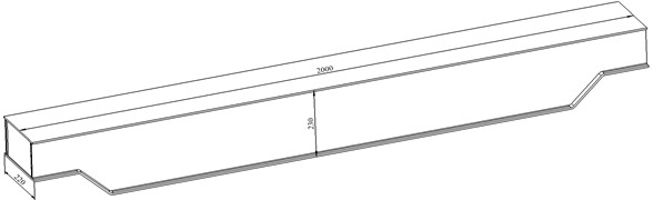
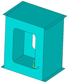
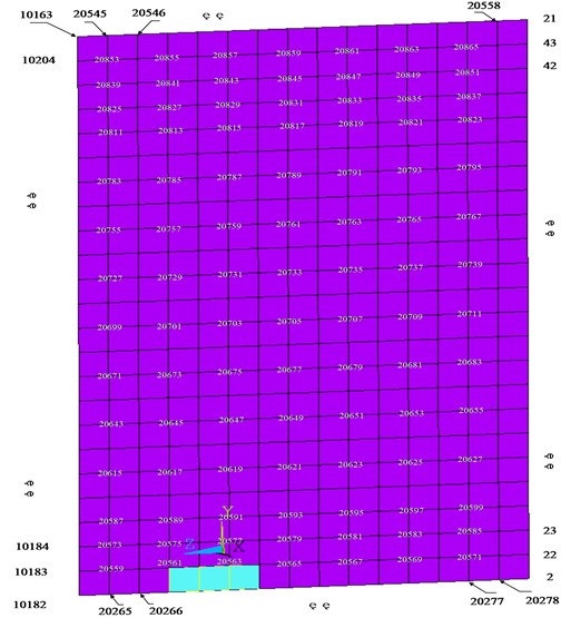
In order to verify the layout method of crane sensors for multi-level damage identification, the forward modeling was used to drive the logic of reverse identification, and the corrosion damage of the main girder web was simulated by finite element analysis to provide accurate damage baseline data. Then, the location and extent of the damage can be inferred from sensor data at specific points. The length of the main beam is 2000 mm, the width is 220 mm, the height is 230 mm, the material is Q345, the elastic modulus is 2.06×10⁵MPa, and the Poisson’s ratio is 0.3. The main beam structure is shown in Fig. 2.

Fig. 23d model of crane girder

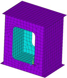
The main beam model is modeled using shell elements with a mesh size of 10 mm. There are two kinds of damage simulation: one is to simulate the damage by reducing the cross-sectional area of the structure; the other is to simulate the damage by changing the elastic modulus of the local material. Three elements 20739,20762 and 20785 were randomly selected to reduce their elastic modulus to 70 % of the original elastic modulus, and the corrosion damage of the structure was simulated as shown in Fig. 3.

Fig. 3Finite element model of corrosion damage

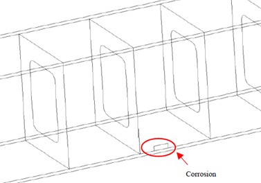
a) Location map of corrosion damage

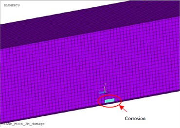
b) Finite element model of corrosion damage

3.1. Sensor placement in the primary phase

From the perspective of geometry, the diaphragm divides the crane girder structure into 17 intervals, as shown in Fig. 4, so it can be decomposed into 17 different identification regions by using the position of the diaphragm in damage identification.

By using joints 12187, 15768, 15302, 11570, 11223, 10876, 10529, 10182, 2, 353, 704, 1055, 1406, 5176, 5648 and 2037, the main girder is divided into Area 1, Area 2, ..., up to Area 15. The boundary points of each region are selected as the accelerometer placement points, and the sensor placement points are shown in Fig. 5.

The natural frequencies of the structure without damage and with corrosion damage are calculated respectively. The results of finite element analysis are shown in Fig. 6 and Fig. 7.

Fig. 4Main beam zoning diagram

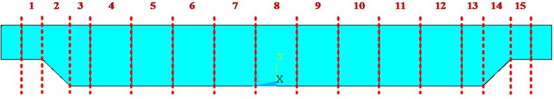
Fig. 5Sensor layout in each area (frequency response output node)

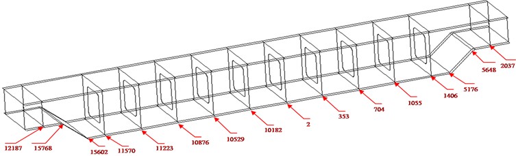
Fig. 6First-order modal diagram without damage

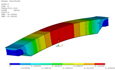
a) Undamaged first mode nephogram

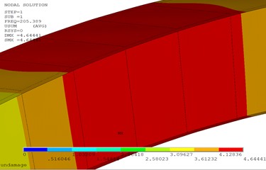
b) Local diagram of undamaged first-order mode

Fig. 7First-order modal diagram of corrosion damage

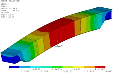
a) First mode Nephogram of corrosion damage

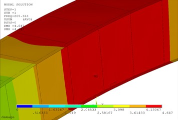
b) First mode local diagram of corrosion damage

Table 1 presents the natural frequencies of the structure and their variations under three different conditions. The data indicate that corrosion damage has a relatively noticeable influence on the natural frequencies in the first ten modes, with the frequency differences reaching 0.12 Hz and 0.13 Hz for the fifth and sixth modes, respectively. Theoretically, such frequency variations can serve as a basis for identifying structural corrosion damage. In practical engineering environments, however, such minor frequency shifts are easily masked by environmental noise and other interference factors. Consequently, damage identification methods relying solely on frequency changes are difficult to apply effectively in practice, revealing the limitations of depending only on frequency variations for damage diagnosis.

Fig. 8Frequency response diagram of x, y, z axis without damage

a) Undamaged $X$ -axis frequency response diagram

b) Undamaged $X$ -axis frequency response diagram (local)

c) Undamaged $Y$ -axis frequency response diagram

d) Undamaged $Y$ -axis frequency response diagram (local)

e) Undamaged $Z$ -axis frequency response diagram

f) Undamaged $Z$ -axis frequency response diagram (local)

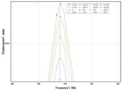
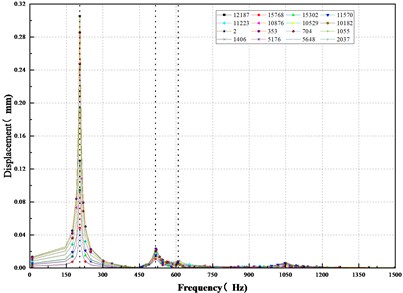
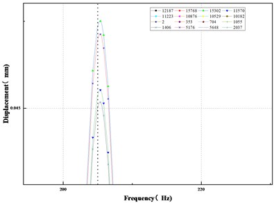
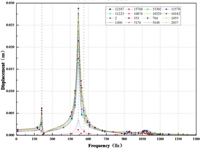
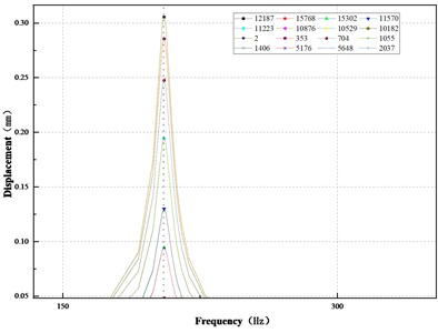
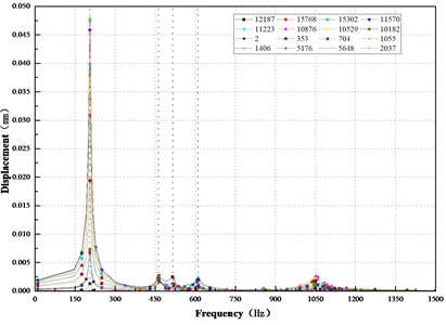
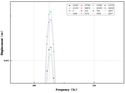
Fig. 8 presents the frequency response curves of the structure at selected measuring points under the undamaged condition. As shown in Fig. 8(a), the displacement response in the $X$ -direction peaks at 516.54 Hz, with a secondary peak occurring at 205.39 Hz. From Fig. 8(c), it can be observed that in the $Y$ -direction, the most pronounced displacement response appears at 212.34 Hz, followed by a secondary peak at 516.54 Hz. According to Fig. 8(e), the $Z$ -direction exhibits its maximum displacement response at 212.34 Hz. Additionally, similar displacement amplitudes are observed at 462.17 Hz, 516.54 Hz, and 609.77 Hz, suggesting that these frequencies exert comparable excitation effects on the vibration in the $Z$ -direction.

Fig. 9Frequency response diagram of x, y, z axis of corrosion damage

a) Corrosion damage $X$ -axis frequency response diagram

b) Corrosion damage $X$ -axis frequency response diagram (local)

c) Corrosion damage $Y$ -axis frequency response diagram

d) Corrosion damage $Y$ -axis frequency response diagram (local)

e) Corrosion damage $Z$ -axis frequency response diagram

f) Corrosion damage $Z$ -axis frequency response diagram (local)

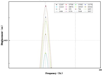
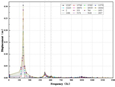
Fig. 9 shows the frequency response of the structure with corrosion damage at specified nodes. As illustrated in Fig. 9(a), the $X$ -direction exhibits a peak displacement at 516.62 Hz and a distinct sub-peak at 205.36 Hz, consistent with the response pattern observed in the undamaged state. However, minor frequency shifts are present across all resonance frequencies, reflecting the influence of corrosion damage on structural stiffness characteristics.

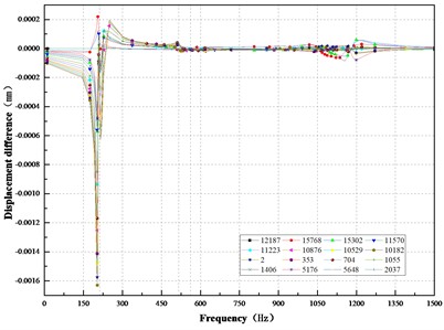
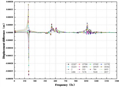
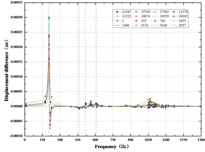
Fig. 10Frequency response difference curves of x, y, z axis of corrosion damage

a) Corrosion damage $X$ -axis frequency response difference curve

b) Corrosion damage $X$ -axis frequency response difference curve

c) Corrosion damage $Y$ -axis frequency response difference curve

d) Corrosion damage $Y$ -axis frequency response difference curve

d) corrosion damage $Z$ -axis frequency response difference curve

f) Corrosion damage $Z$ -axis frequency response difference curve

Fig. 9(c) indicates that in the $Y$ -direction, the displacement response reaches its maximum at 212.33 Hz, with a secondary resonance occurring at 462.19 Hz. According to Fig. 9(e), the $Z$ -direction shows the most significant displacement response at 212.33 Hz, while similar displacement amplitudes are observed at 462.19 Hz, 516.62 Hz, and 609.64 Hz, forming a typical multi-peak resonance pattern. Compared to the undamaged condition, corrosion damage leads to slight but identifiable shifts in resonant frequencies in all directions, along with varying degrees of change in displacement amplitude. These results demonstrate that corrosion not only induces a systematic shift in resonant frequencies but also causes a redistribution of displacement response amplitudes across the structure.

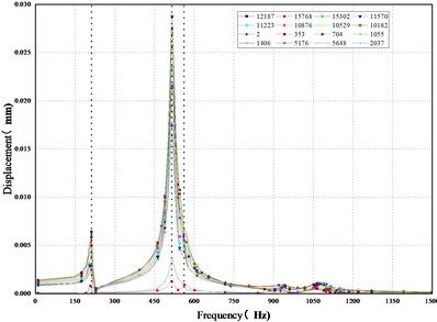
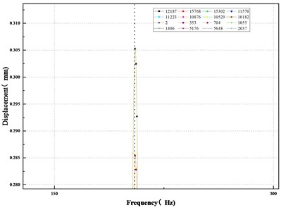
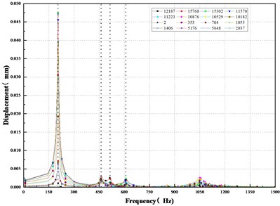
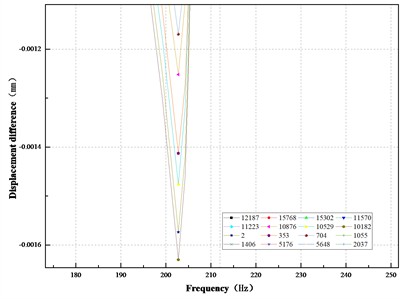
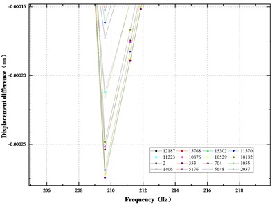
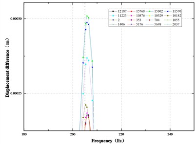
Fig. 10 presents the frequency response difference curves of the structure at specified measuring points under corrosion damage. The results indicate that the nodal displacement response differences peak at the first six frequencies: 205.36 Hz, 212.33 Hz, 462.19 Hz, 516.62 Hz, 562.15 Hz, and 609.64 Hz. In terms of directional distribution, the frequency response differences are most pronounced in the $X$ -direction at nodes 10182 and 10529, whereas nodes 2037 and 12187 show no response. In the $Y$ -direction, nodes 10182 and 10529 exhibit significant differences at 205.36 Hz. In the $Z$ -direction, nodes 15302 and 11750 are more sensitive at 205.36 Hz, while nodes 5176 and 1406 respond notably at 212.33 Hz. Structural damage can thus be identified via the frequency response displacement differences at the joints, with differences in the $X$ - and $Y$ -directions being correlated to the damage area. Nodes 12187 and 2037 are insensitive to damage and may be excluded from sensor placement consideration.

Table 1Structure frequency and frequency difference in different cases

Modal order	Undamaged (Hz)	Corrosion damage
Modal order	Undamaged (Hz)	Frequency (Hz)	Difference in frequency (Hz)
1	205.39	205.36	0.03
2	212.34	212.33	0.01
3	462.17	462.19	0.02
4	516.54	516.62	0.08
5	562.27	562.15	0.12
6	609.77	609.64	0.13
7	866.28	866.27	0.01
8	878.86	878.86	0
9	931.85	931.78	0.07
10	1050	1049.9	0.1

3.2. Damage area identification in intermediate stage

Node 12187 and node 2037 are not sensitive to the corrosion damage of the structure, and the sensor is not considered when it is installed, so the remaining nodes are further selected to locate the damage area. Based on the displacement frequency response amplitude change matrix of each output node before and after damage $D_{n m}$ :

20

D_{n m}^{x} = |\begin{matrix} - 1.76 \times 1 0^{- 5} & \dots & - 1.15 \times 1 0^{- 5} \\ ⋮ & ⋱ & ⋮ \\ 5.66 \times 1 0^{- 6} & \dots & 1.06 \times 1 0^{- 5} \end{matrix}|,

21

D_{n m}^{y} = |\begin{matrix} 1.7 \times 1 0^{- 6} & \dots & - 5.7 \times 1 0^{- 7} \\ ⋮ & ⋱ & ⋮ \\ - 4.9 \times 1 0^{- 7} & \dots & 6.4 \times 1 0^{- 7} \end{matrix}|,

22

D_{n m}^{z} = |\begin{matrix} 2.8 \times 1 0^{- 6} & \dots & 6.0 \times 1 0^{- 7} \\ ⋮ & ⋱ & ⋮ \\ 2.4 \times 1 0^{- 7} & \dots & 1.0 \times 1 0^{- 7} \end{matrix}| .

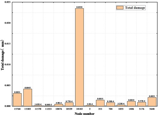
The matrix of amplitude variations is processed column-wise: only the maximum value in each column is retained, while all other elements are set to zero. This modified matrix is subsequently summed along its rows, yielding the resultant vector shown in Table 2. Each element of this vector can be used as a damage identification index. The damage location is determined as the region adjacent to the node associated with the maximum element therein.

Table 2Damage identification vector of corrosion damage

Sum of node damage	$d_{v 1}$	$d_{v 2}$	$d_{v 3}$	$d_{i a}$
15768	0.308×10^-2	0	0	0.308×10^-2
15302	0.647×10^-3	0.036×10^-4	0.035×10^-1	0.415×10^-2
11570	0	0.157×10^-3	0.393×10^-5	0.161×10^-3
11223	0	0.884×10^-4	0	0.884×10^-4
10876	0.142×10^-3	0.348×10^-3	0	0.049×10^-2
10529	0.654×10^-4	0.811×10^-3	0	0.877×10^-3
10182	0.0195	0.224×10^-2	0.183×10^-2	0.235×10^-1
2	0	0.609×10^-5	0.214×10^-3	0.022×10^-2
353	0.535×10^-3	0.956×10^-3	0	0.149×10^-2
704	0.502×10^-3	0.353×10^-3	0.435×10^-5	0.859×10^-3
1055	0.532×10^-4	0.269×10^-3	0	0.323×10^-3
1406	0	0.119×10^-2	0.898×10^-6	0.119×10^-2
5176	0.786×10^-3	0.043×10^-3	0.129×10^-3	0.957×10^-3
5648	0.194×10^-2	0.153×10^-3	0	0.0021

As shown in Fig. 11, the maximum damage occurs at node 10182, while damage at other nodes is relatively negligible. Therefore, it can be concluded that the damage is located near node 10182. Given that node 10529 exhibits more prominent damage than node 2, the actual damage is closer to node 10529. With reference to Fig. 4, it can be inferred that the girder structure is prone to cracking in either region 7 or region 8.

Fig. 11Comparison diagram of each node damage index

3.3. Advanced stage of precise sensor placement

For accurate spatial localization of structural damage, once its existence is preliminarily confirmed, the flexibility difference analysis method is applied for further identification. To improve the accuracy and reliability of damage localization, additional sensors are installed in the identified region to monitor local flexibility variations. Examples include vibration measurement systems for tracking displacement and distributed optical fiber sensors for measuring strain. The finite element model of the nodal surrounding region is extracted in Fig. 12, and the corresponding model for web structural damage is presented in Fig. 13.

Fig. 12Finite element model of local area

a) 3D model of main beam

b) Main beam mesh model

Fig. 13Finite element model of web structure damage

In the finite element processing, the node number in the corresponding graph is represented by the matrix $N_{n}$ , and the element number in the corresponding graph is represented by the matrix $E_{n}$ :

23

N_{n} = [\begin{matrix} 10163 & 20545 & 20546 & \dots & 21 \\ 10204 & 20853 & 20854 & \dots & 43 \\ 10203 & 20839 & 20840 & \dots & 42 \\ ⋮ & ⋮ & ⋮ & ⋱ & ⋮ \\ 10182 & 20265 & 20266 & \dots & 2 \end{matrix}] .

For the thin plate structure, the influence of damage on the tangential ( $Y$ axis, $Z$ axis) stiffness is much smaller than that on the normal ( $X$ axis) stiffness. The first six natural frequencies of the structure $ω_{i}$ ( $i =$ 1, 2, ... , 6) are shown in Table 1, according to Eq. (18) , the first six order normal displacement vectors $φ_{i}$ ( $i =$ 1,2, ... , 6) of the structure are calculated, according to Eq. (19) , the flexibility matrix Fa of the first six modes can be calculated:

24

F = [\begin{matrix} 5.16 \times 1 0^{- 4} & 5.16 \times 1 0^{- 4} & 5.17 \times 1 0^{- 4} & \dots & 5.07 \times 1 0^{- 4} \\ 5.12 \times 1 0^{- 4} & 5.13 \times 1 0^{- 4} & 5.13 \times 1 0^{- 4} & \dots & 5.03 \times 1 0^{- 4} \\ 5.08 \times 1 0^{- 4} & 5.09 \times 1 0^{- 4} & 5.10 \times 1 0^{- 4} & \dots & 4.99 \times 1 0^{- 4} \\ ⋮ & ⋮ & ⋮ & ⋱ & ⋮ \\ 5.15 \times 1 0^{- 4} & 5.52 \times 1 0^{- 4} & 5.52 \times 1 0^{- 4} & \dots & 5.45 \times 1 0^{- 4} \end{matrix}] .

According to the order of nodes and elements, the heat map and the maximum normalized damage location map of the web are constructed. The damage location map is shown in Fig. 14.

Fig. 14Result of corrosion damage localization

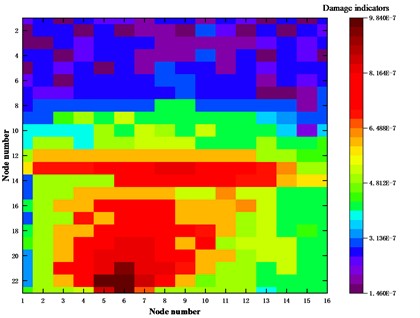
a) Thermal diagram for locating corrosion damage in web structure

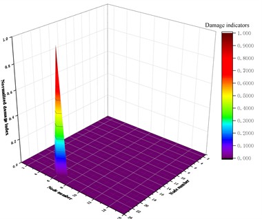
b) Surface diagram for locating corrosion damage in web structure

The identified location of the corrosion damage is largely consistent with the preset damage location in the simulation. As shown in Fig. 14(a), the damage index near the damaged area is significantly higher than that in undamaged regions. The nodes with the largest damage indices are the 5th, 6th, and 7th nodes, which correspond to the predefined units 20739, 20762, and 20785, respectively. Fig. 14(b) further indicates that the maximum damage index occurs at the 6th node, where unit 20762 is situated between the other two units. These results demonstrate that corrosion damage can be accurately identified by deploying vibration sensors to monitor the vibration displacement of the web in regions with significant flexibility differences.

4. Conclusions

The crane structure is characterized by its large scale and complex cross-sectional forms. The effectiveness of the sensor layout scheme in covering key areas and accurately identifying structural damage directly determines the practical application value of the structural health monitoring system. The main conclusions of this study are as follows:

1) In the preliminary identification stage, based on the analysis of displacement response characteristics of corrosion damage under different frequencies, it was found that the displacement response differences of each node in the corrosion-damaged structure exhibited significant distribution characteristics under the first six modal frequencies, and the displacement response differences of each node were most pronounced in the first modal. Initial damage can be identified through the frequency response displacement difference at the joints, and the differences in the $X$ - and $Y$ -directions show a clear correlation with the damage location. The study confirms that nodes 12187 and 2037 are insensitive to damage and can be excluded from the sensor layout, thereby achieving preliminary optimization of measurement points.

2) In the intermediate identification stage, the influence of damage on the displacement frequency response amplitude is effectively enhanced by applying weighted superposition of displacement differences at the same node across different frequencies, enabling accurate identification of the damaged area. The results indicate a negative correlation between the spatial distance from a joint to the damage location and the corresponding displacement variation. Through collaborative analysis of damage vectors in the $X$ -, $Y$ -, and $Z$ -directions, the identification of the damage region can be significantly improved. Although the maximum corrosion damage value is also observed at node 10182, its area of influence is closer to node 10529, primarily distributed in vulnerable region 7 or 8.

3) In the advanced identification stage, a correction algorithm based on displacement flexibility difference was adopted to achieve precise localization of damage points and optimal arrangement of sensors. The research results show that the damage index near the damaged area is significantly higher than that of the undamaged area. The points with higher damage index are consistent with the designated units 20739, 20762, and 20785. The maximum damage index is located at unit 20762, which is in the middle of the three preset damaged units. Corrosion damage can be accurately identified by arranging vibration sensors to monitor the vibration displacement of the web plate and then accurately identifying corrosion damage through changes in the displacement flexibility difference of the web plate.

References

D. Wu, “Research on optimized layout of bridge sensors based on MAC stepwise addition and subtraction algorithm,” Journal of Vibroengineering, Vol. 24, No. 8, pp. 1486–1501, Dec. 2022, https://doi.org/10.21595/jve.2022.22574

Publisher
S. Hu, Z. Ding, S. Liu, Q. Wei, D. Novák, and M. Cao, “Structural damage detection by progressive continuous wavelet transform and singular value decomposition of noisy mode shapes,” Journal of Vibroengineering, Vol. 27, No. 7, pp. 1240–1260, Nov. 2025, https://doi.org/10.21595/jve.2025.24920

Publisher
G. Sha, M. Cao, W. Xiao, M. Radzieński, and H. Zuo, “Damage localization in beams based on the analysis of modal parameters,” Vibroengineering Procedia, Vol. 46, pp. 48–53, Nov. 2022, https://doi.org/10.21595/vp.2022.22999

Publisher
J. Chen and F. Xiong, “Curvature mode shapes-based damage identification method,” (in Chinese), Journal of Wuhan University of Technology, Vol. 29, No. 3, pp. 99–102, Jan. 2007, https://doi.org/10.3321/j.issn:1671-4431.2007.03.028

Publisher
H. Chen and D. J. Yu, “Study on the damage detection in the beam bridge using changes in curvature mode shape,” (in Chinese), Journal of Highway and Transportation Research and Development, Vol. 21, No. 10, pp. 55–57, Jan. 2004, https://doi.org/10.3969/j.issn.1002-0268.2004.10.015

Publisher
M. Khan, S. Mahato, D. Eidukynas, and T. Vaitkunas, “Influence determination of damage to mechanical structure based on modal analysis and modal assurance criterion,” Vibroengineering Procedia, Vol. 42, pp. 27–32, May 2022, https://doi.org/10.21595/vp.2022.22554

Publisher
X. Wang and Z. Zhao, “Study of structural damage identification based on the proportional flexibility matrix and improved modal curvature method,” (in Chinese), Shanxi Architecture, Vol. 43, No. 19, pp. 46–48, Jan. 2017, https://doi.org/10.13719/j.cnki.cn14-1279/tu.2017.19.024

Publisher
S. Tang et al., “Structural damage identification method based on curvature norm difference of modal flexibility matrix,” (in Chinese), Chinese Journal of Applied Mechanics, Vol. 37, No. 3, pp. 982–989, 2020.

Search CrossRef
V. B. Dawari and G. R. Vesmawala, “Modal curvature and modal flexibility methods for honeycomb damage identification in reinforced concrete beams,” Procedia Engineering, Vol. 51, pp. 119–124, Jan. 2013, https://doi.org/10.1016/j.proeng.2013.01.018

Publisher
M. Zhang, X. Peng, Y. Li, Z. Wang, J. Zhu, and J. Zhang, “Study on the structural damage detection method using the flexibility matrix,” Latin American Journal of Solids and Structures, Vol. 21, No. 6, Jan. 2024, https://doi.org/10.1590/1679-78257966

Publisher
K. Zhou, Y. Liu, and C. Xu, “Damage identification of tower crane structure based on flexibility curvature,” (in Chinese), Journal of University of Shanghai for Science and Technology, Vol. 44, No. 6, pp. 562–567, Jan. 2021, https://doi.org/10.13255/j.cnki.jusst.20210822002

Publisher
T. Wang and Z. Wan, “An optimized layout approach of the sensor placement for structural parameter identification,” (in Chinese), Machinery Design and Manufacture, No. 4, pp. 17–20, Jan. 2024, https://doi.org/10.19356/j.cnki.1001-3997.20241121.027

Publisher
J. Zhou et al., “Damage identification based on modal strain energy formulated by strain modes,” (in Chinese), Journal of Vibration, Measurement Diagnosis, Vol. 39, No. 1, pp. 25–31, Jan. 2019, https://doi.org/10.16450/j.cnki.issn.1004-6801.2019.01.004

Publisher
Z. Niu et al., “Statistical damage identification of structures using incomplete FRF data,” (in Chinese), Chinese Journal of Applied Mechanics, Vol. 38, No. 1, pp. 192–199, 2020.

Search CrossRef
J.-C. Chen and J. A. Garba, “On-orbit damage assessment for large space structures,” AIAA Journal, Vol. 26, No. 9, pp. 1119–1126, Sep. 1988, https://doi.org/10.2514/3.10019

Publisher
S. Wang, X. Long, H. Luo, and H. Zhu, “Damage identification for underground structure based on frequency response function,” Sensors, Vol. 18, No. 9, p. 3033, Sep. 2018, https://doi.org/10.3390/s18093033

Publisher
T. Qi, Z. Hou, and L. Yu, “Structural damage identification based on dual sensitivity analysis from optimal sensor placement,” Journal of Infrastructure Intelligence and Resilience, Vol. 3, No. 3, p. 100110, Sep. 2024, https://doi.org/10.1016/j.iintel.2024.100110

Publisher
T. H. Loutas and A. Bourikas, “Strain sensors optimal placement for vibration-based structural health monitoring. The effect of damage on the initially optimal configuration,” Journal of Sound and Vibration, Vol. 410, pp. 217–230, Dec. 2017, https://doi.org/10.1016/j.jsv.2017.08.022

Publisher
Y.-F. Zou, Y.-H. Su, X.-D. Lu, X.-H. He, and C.-Z. Cai, “Structural damage detection based on model reduction and response reconstruction,” Journal of Central South University, Vol. 32, No. 11, pp. 4439–4462, Jan. 2026, https://doi.org/10.1007/s11771-025-6105-1

Publisher
H. Yang, B. Yan, Y. Gao, H. Deng, X. Wu, and C. Wu, “Global damage identification method based on multi-source signals and ST-GNN for frame structures,” International Journal of Structural Stability and Dynamics, Jan. 2026, https://doi.org/10.1142/s0219455427501318

Publisher
G. F. Gomes and V. D. Takano, “Strain-based identification of multiple damages in plate-like structures using artificial intelligence and metaheuristic optimization,” Machine Learning for Computational Science and Engineering, Vol. 2, No. 1, pp. 5–5, Feb. 2026, https://doi.org/10.1007/s44379-025-00052-w

Publisher

About this article

Received

November 4, 2025

Accepted

March 17, 2026

Published

May 16, 2026

SUBJECTS

Fault diagnosis based on vibration signal analysis

DOI

https://doi.org/10.21595/jve.2026.25812

Keywords

crane

damage identification

optimal sensor placement

structural health monitoring

Acknowledgements

The financial supports received from National Key R&D Program of China (2024YFC3014900).

Data Availability

The datasets generated during and/or analyzed during the current study are available from the corresponding author on reasonable request.

Author Contributions

Hui Jin: conceptualization, funding, acquisition, methodology, writing-review and editing. Keqin Ding: conceptualization, project administration, supervision. Guansi Liu: methodology, investigation, software, validation, writing-original draft preparation

Conflict of interest

The authors declare that they have no conflict of interest.

This is an open access article distributed under the Creative Commons Attribution License, which permits unrestricted use, distribution, and reproduction in any medium, provided the original work is properly cited.

G. Liu, H. Jin, and K. Ding, “Sensor placement method for crane structural health monitoring based on multi-level damage identification,” Journal of Vibroengineering, Vol. 28, No. 2, –17, May 2026, https://doi.org/10.21595/jve.2026.25812

Copy Extrica

Copied to clipboard!

TY  - JOUR
DO  - 10.21595/jve.2026.25812
UR  - https://doi.org/10.21595/jve.2026.25812
TI  - Sensor placement method for crane structural health monitoring based on multi-level damage identification
T2  - Journal of Vibroengineering
AU  - Liu, Guansi
AU  - Jin, Hui
AU  - Ding, Keqin
PY  - 2026
DA  - 2026/05/16
PB  - Extrica
VL  - 28
IS  - 2
SN  - 1392-8716
SN  - 2538-8460
ER  - 

Copy Ris

Copied to clipboard!

@article{doi_10.21595/jve.2026.25812,
  title = {Sensor placement method for crane structural health monitoring based on multi-level damage identification},
  author = {Liu, Guansi and Jin, Hui and Ding, Keqin},
  journal = {Journal of Vibroengineering},
  year = {2026},
  month = {5},
  volume = {28},
  number = {2},
  doi = {10.21595/jve.2026.25812},
  url = {https://doi.org/10.21595/jve.2026.25812},
  publisher = {Extrica},
  issn = {1392-8716},
  eissn = {2538-8460},
}

Copy Bibtex

Copied to clipboard!

[1]G. Liu, H. Jin, and K. Ding, “Sensor placement method for crane structural health monitoring based on multi-level damage identification,” Journal of Vibroengineering, May 2026, doi: 10.21595/jve.2026.25812.

Copy IEEE

Copied to clipboard!

Liu, Guansi, Hui Jin, and Keqin Ding. “Sensor placement method for crane structural health monitoring based on multi-level damage identification.” Journal of Vibroengineering 28, no. 2 (2026). https://doi.org/10.21595/jve.2026.25812.

Copy Chicago

Copied to clipboard!

Sensor placement method for crane structural health monitoring based on multi-level damage identification

Abstract

1. Introduction

2. Sensor placement method for multi-level progressive damage identification

2.1. Initial stage: sensor placement based on region division

2.2. Intermediate stage: damage area identification based on displacement frequency response difference correction

2.3. Advanced stage: precise sensor placement for node-level damage identification

3. Simulation analysis of crane girder structure

3.1. Sensor placement in the primary phase

3.2. Damage area identification in intermediate stage

3.3. Advanced stage of precise sensor placement

4. Conclusions

References

About this article

Related Articles