Abstract
The difference in the location and number of sensors induces the acquisition effect of structural state information in the bridge health monitoring system to a certain extent, which is also one of the most difficult problems restricting the development of bridge health monitoring technology. Based on the Modal Assurance Criterion, this paper took a cantilever simply supported beam as an example and adopted the Effective Independence method, Kinetic Energy method and QR decomposition method to optimize a sensor layout. Taking the number of sensors as 5, the layout and MAC matrix factors were analyzed by comparing the MAC matrix and its distribution diagrams obtained by different methods. The results showed that the stepwise subtraction method based on QR decomposition was the best. And by changing the number of sensor, it was found that the optimal number of sensor was 9. It was also found that the existing methods had the shortcomings of over-reliance on the selection of initial measuring points. In order to improve this defect, cyclic iteration of stepwise addition and subtraction was introduced, and an optimal layout method based on the stepwise addition and subtraction of the number of sensors was proposed. Through screening and optimization of this method, the average off-diagonal element in the calculation example was reduced from 0.118 to 0.006 to achieve the satisfactory optimization effect. At the same time, this method was employed to optimize the layout of a concrete continuous rigid-frame bridge with 9 and 19 sensors, and the results showed that the sensor layout was more uniform. Therefore, the proposed method provides the opportunity to obtain fair optimization results and to have a considerable engineering application value.
Highlights
- An optimal layout method of measuring points that stepwisely increase and decrease the number of sensors was proposed.
- The existing sensor optimization layout methods have certain limitations because they rely too much on the selection of the initial measuring points.
- The measuring point optimization method based on matrix QR decomposition could greatly reduce the value of the average off-diagonal element and improve the effect of sensor optimization.
1. Introduction
Sensor layout is one of the most important links in bridge health monitoring system [1-3]. The state monitoring system of the overall bridge structure can be established by laying different types and numbers of sensors at key positions on the surface or inside the structure [2]. A complete acquisition system composed of various sensors can present the environmental impact (temperature, humidity and wind level), load conditions and overall or local dynamic and static characteristic parameters of the bridge so that the real time operation status can be monitored [4].
The monitoring of environmental impact, load condition and structural static characteristic parameters can be processed by placing a few sensors in the key parts of the structure to obtain relatively accurate data. However, due to the different functions and positions of each bridge component, its geometric characteristics, material properties and the response of the external environment, such as ground motion, strong wind, torrential rain, etc., the dynamic characteristic parameters of the structure are quite discrepant. Therefore, how to obtain the expected structural dynamic parameters for real-time monitoring of the bridge through a reasonable sensor layout so as to analyze the structure state is one of the most tough problems in health monitoring [5-7]. And the optimal sensor layout is the key link in this problem.
The sensor layout problem is essentially a 0-1 knapsack optimization problem. The maximum efficiency of the sensor layout system can be obtained through the reasonable layout taking into account all the configurable degrees of freedom and the number of sensors [8]. In practical engineering applications, the problem of optimal sensor layout is not only affected by the structure itself, i.e. sensor layout, quantity, measurability of the dynamic characteristics, but also by economic factors, i.e. sensor price, construction and design cost of sensor placement, etc., and the environment factors, i.e. underwater structures, the influence of ultra-high artifacts, etc. Therefore, it is extremely important to study how to optimize the layout and the number of sensors [9-11].
In this paper, through a series of researches and analyses on the evaluation criteria and layout methods, an optimal layout method based on the stepwise addition and subtraction of the number of sensors was proposed, and a simple supported cantilever beam was used to verify this method. The results showed that the orthogonality of structural modal information reflected by a few measuring points was better than that of the traditional method. And then it was applied to the optimal layout of sensors of a continuous rigid frame bridge and provided a theoretical reference for the layout of on-site measuring points, which verified its great practicability.
2. Modal assurance criterion for optimal layout of measuring points
The different orders of acceleration, displacement and strain in the overall structural element have a certain orthogonality, and for some nodes, the spatial angle of the modal vector is relatively large to be used for evaluating the modal position vector of each node. In view on this, Thomas G. et al. proposed the Modal Assurance Criterion (MAC) matrix method [12], through which the corresponding assurance criterion can be obtained. The MAC can provide a reliable suggestion on whether to arrange sensors at the measuring points, and a small value in the non-diagonal element of the matrix can be used to optimize the layout of the measuring points, namely:
where is the th order modal vector of the structure, and is the th order modal vector of the structure. The range of is [0, 1], 0 means that the vectors of the two measurement points are completely orthogonal, and 1 means that the vectors of the two measurement points are completely correlated and not orthogonal. Therefore, for the off-diagonal elements of a MAC matrix, its numerical magnitude is directly proportional to the vector correlation.
3. Optimal layout method of measuring points
3.1. Effective independence method (EIM)
The basic idea of the traditional EIM [13-15] is to start from the vibration modes of the target structure, such as acceleration, strain and displacement, and make use of the characteristics of the composite mode matrix to remove the measuring points from the original measuring point group of the structure. Based on the minimum error criterion, the Fisher information matrix is optimized and improved by sequentially deleting the degrees of freedom of the measuring points that contribute the least to the Fisher information matrix. Via the idempotent form of the composite mode matrix, the most appropriate number of sensors is selected to obtain the linear independent mode shape of the target structure as much as possible, so as to distinguish preferably the real state of the target structure.
matrix is an idempotent matrix, which means that , its eigenvalue is 1 or 0, and the th element on its diagonal represents the contribution of the th degree of freedom or the test point to the matrix or rank (trace), that is, the contribution to the matrix [16]. Therefore, represents the effective independence distribution of the set of candidate sensor locations. The element on the diagonal of represents the linearly independent contribution of the corresponding sensor candidates to the modal matrix, namely:
When 0, it means that the corresponding mode cannot be identified at the corresponding measuring point . When 1, it means that the corresponding measuring point on the th measuring point is a key measuring point and cannot be excluded. The priority order of each candidate point is sorted according to the value of .
The iterative algorithm is used to eliminate the measuring points with the smallest each time, and then the next iteration is performed until the corresponding number of sensor layout is reached. The effective independence method can maintain the linear independence of the modal matrix and the integrity of the Fisher information matrix as much as possible through this iterative algorithm, and can basically retain the modal characteristics of the original structure, so that the optimal modal characteristics can be obtained from the limited modal data.
3.2. Kinetic energy method (KEM)
The Kinetic Energy Method [17-18] is based on the connection between the modal strain energy and the response in the degrees of freedom. The modal strain energy curve is drawn by the strain modal values of each degree of freedom in the vibration response. According to the strain values of each degree of freedom, sensors are arranged in the place where the strain is large so as to achieve the purpose of structural state identification.
The Kinetic Energy Matrix (KEM), proposed by G. Heo in 1997 [19], uses the quality matrix to weigh the Fisher information matrix , and is defined as follows:
Via orthogonally decomposing of the mass matrix , the following equation can be obtained:
Substituting Eq. (4) into Eq. (3), the following equation can be obtained:
If to suppose , then:
The modal kinetic energy of each test degree of freedom can be obtained through Eq. (6), :
Therefore, after calculating , the modal kinetic energy of each degree of freedom can be obtained. Then the sensor position can be optimized according to the iterative optimization method for deleting the smallest diagonal element.
Based on the modal kinetic energy characteristics, the sensor configuration using this method has fair noise immunity. However, the accuracy of this method is closely related to the meshing precision of the finite element model, and the element meshing thickness may affect the distance of the sensor distribution, which has a great influence on the measured parameters that truly reflect the structural state [20].
3.3. MAC method based on QR decomposition
The choice of the initial position of the measuring point will greatly affect the working time consumption and accuracy of the later position optimization. Therefore, when using the MAC method to optimize the layout of sensors, the selection of initial measurement points is very important. The more reasonable the selection of preliminary measuring points will be, the simpler the optimization of later measuring points will be.
Therefore, the concept of QR decomposition was introduced in order to optimize the selection of initial measuring points. Using the effective independence method, the maximum norm was determined for Fisher information matrix as:
Therefore, after selecting an appropriate , a Fisher information matrix that satisfies the conditions can be obtained. And QR decomposition method can be obtained by norm processing.
Let us suppose that the subset of measurable degrees of freedom of a finite element model is , , then the number of measuring points and , that is, the matrix is a full rank matrix. Since the column pivot element selects a subset of the column vector group for QR decomposition, and the row space characteristic of the measurement vector is utilized. Therefore, QR decomposition of its column pivot can be obtained as follows:
where , , , are Permutation Matrices. The extraction of subset with larger norm in Φ row vector set provided initial measuring points for the MAC method [21].
After selecting the initial measuring points, their layout could be optimized. In this stage, the sequential method is mainly used for processing, and the traditional sequential method can be subdivided into two methods, that is, stepwise addition method and stepwise subtraction method.
3.3.1. Stepwise addition method [22]
The stepwise addition method is an iterative process of adding the number of sensors in the optimized area. With the maximum off-diagonal elements reaching the preset threshold (typically, < 0.25) as the optimization goal, this method takes the preliminary measuring points selected by QR decomposition as the basis of optimizing the measuring point area, and selects the measuring points one by one from the remaining optional measuring point set and accumulates them to the optimized measuring point area for the MAC matrix analysis, and ultimately figures out the appropriate number of sensors.
From Eq. (1), the largest off-diagonal element of the MAC matrix of the th and th order modes of can be calculated as:
For the MAC matrix of the stepwise addition method, it can be obtained as follows:
Analysis shows that for , the numerator is always greater than 0. When the numerator 0, the is also greater than 0. So it becomes possible to reduce the largest off-diagonal element.
The objective function of stepwise addition method can be defined as follows:
By adjusting the objective function , the largest off-diagonal element can reach the preset threshold (such as 0.25).
3.3.2. Stepwise subtraction method [23]
Stepwise subtraction is an iterative process of subtracting the number of sensors in the optimized area. This method is based on the sequence of the preliminary measuring points selected by QR decomposition, and the measuring point areas with more than the number of optimized sensors are selected as the measuring point set, from which the unsuitable measuring points are selected one by one for deletion. After subtracting, the modal assurance analysis is carried out on the modal matrix of the remaining preset number of sensors to reduce the maximum off-diagonal element in the MAC matrix for the purpose of optimization, and the most suitable sensor location and number can be obtained by selecting the most suitable measuring point area:
By analysis, for , the numerator is always greater than 0. When the numerator 0, the is also less than 0. So it becomes possible to increase the largest off-diagonal element.
The objective function of the stepwise subtraction method can be defined as follows:
Through adjusting the objective function , the minimum off-diagonal element can reach the preset threshold (such as 0.25).
4. Numerical case
4.1. Simulation model
In order to verify the above measuring point optimization method, this paper selected a cantilever simply supported beam model [24] for the optimization analysis of the measuring point layout. The first five-order natural frequency and vertical displacement mode shape of the structure were extracted as the basic parameters for the optimization of the measuring point position. The dimensions and element division of the simply supported beam are shown in Fig. 1, and the first five natural frequencies are listed in Table 1.
Fig. 1Cantilever simply supported beam model and element division (unit: cm)
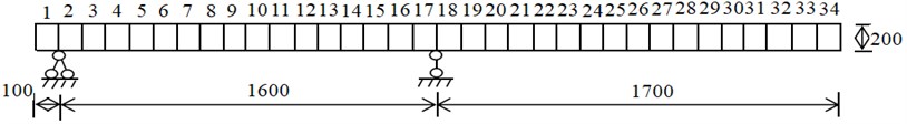
Table 1First five-order frequencies of cantilever simply supported beams
Order | First | Second | Third | Fourth | Fifth |
Frequency / Hz | 1.233 | 6.795 | 10.799 | 24.886 | 31.667 |
4.2. Contribution value solution of effective independence method and kinematic energy method
EIM and KEM methods can be used to obtain effective independent contribution values and relative modal kinetic energy values for different measurement points as shown in Figs. 2(a) and 2(b).
Fig. 2Contribution values for each measuring point
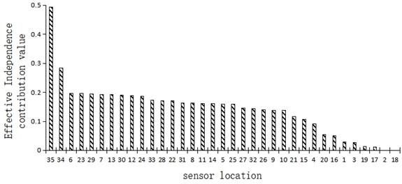
a) Effective independence contribution value
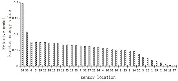
b) Relative modal kinetic energy value
Fig. 2(a) shows the effective independent contribution values for different measuring points of a simply supported cantilever beam. It can be seen that the effective independence of elements 35 and 34 and other cantilever end positions was the strongest, followed by that of elements 6, 7, 23 and 29 and other one-third section positions, and the effective independence of elements 2 and 18 and other fulcrum positions was the weakest.
Fig. 2(b) shows the relative modal kinetic energy values of the simply supported cantilever beams at different measuring points. It can be seen that the relative modal kinetic energy of elements 34 and 33 and other cantilever end positions was the strongest, followed by that of elements 5, 6, 29 and 22 and other one-third section positions, and the relative modal kinetic energy of elements 17 and 18 and other fulcrum positions was the weakest.
It can be seen from the above analysis that the effective independent contribution value and the relative modal kinetic energy value of the cantilever simply supported beam structure generally had a similar distribution trend – the strongest near the cantilever end, followed by the position at the third section, and the weakest near the fulcrum position.
4.3. Comparative analysis of results
4.3.1. MAC matrix comparative analysis
The smaller the off-diagonal element of MAC matrix is, the more independent the position of measuring points is, and the more accurately the real state of the structure can be reflected. In order to compare this matrix with the principle consisting in laying sensors on all elements of a cantilever simply supported beam, the EIM, KEM, stepwise addition method and stepwise subtraction method based on QR decomposition were adopted to select 5 units for laying sensors, and the layout sequence is shown in Table 2.
Table 2Sensor layout of four optimization methods
Layout methods | Sensor layout sequence |
All measuring points layout | All Elements |
EIM | 35E, 34E, 6E, 23E, 29E |
KEM | 34E, 33E, 6E, 5E, 29E |
Stepwise addition of QR decomposition | 35E, 29E, 6E, 13E, 24E |
Stepwise subtraction of QR decomposition | 35E, 6E, 30E, 12E, 24E |
By comparing the four layout sequences listed in Table 2, it is clear that for structures such as cantilever simply supported beams, it was the most important to test the cantilever end and then the one-third and two-thirds section. But different methods also had discrepancies in the layout sequence and position of measuring points.
The MAC matrix, three-dimensional histogram, maximum off-diagonal element and the average off-diagonal element value of the MAC matrix are shown in Table 3.
By comparing the largest off-diagonal element of the MAC matrix in Table 3, it can be seen that the value obtained by the KEM was the largest, namely 0.806; by comparing the average off-diagonal elements of the MAC matrix in Table 3, it can be seen that the value obtained by the EIM was the largest, namely 0.314. In the longitudinal comparison of the maximum and average off-diagonal metadata of MAC matrix in Table 3, when sensors were deployed at all measuring points, the off-diagonal elements of MAC matrix were small, and their maximum and average off-diagonal elements were only 0.008 and 0.004 respectively. This result also verified that the Modal Assurance Criterion could reflect the measuring point layout effect.
By comparing the EIM, KEM, stepwise addition method based on QR decomposition and stepwise subtraction method based on QR decomposition for 5 element positions, the following conclusions can be drawn: both methods based on QR decomposition could promote a satisfactory measuring points layout, especially the stepwise subtraction method; moreover, the off-diagonal element value in the MAC matrix obtained by EIM and KEM was relatively large, which reflected poor measuring points layout.
Therefore, it can be concluded that in case of using EIM and KEM to optimize the layout of measuring points, the number of selected elements should not be too small, otherwise it would be difficult to achieve a satisfactory layout effect. In addition, when EIM was used for layout, only the modal information of each degree of freedom of the structure was considered, while the influence of energy factors was ignored, resulting in poor stability of sensors layout.
Table 3Comparison of effects of different optimization methods
Optimization layout methods | MAC matrix | MAC layout | Largest off-diagonal element value | Average off-diagonal element value | |
All measuring points layout | 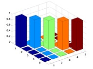 | 0.008 | 0.004 | ||
1 | EIM | 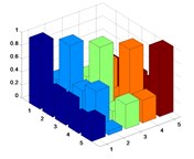 | 0.547 | 0.314 | |
2 | KEM | 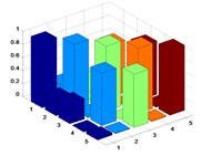 | 0.806 | 0.232 | |
3 | QR decomposition (stepwise addition) | 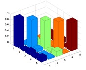 | 0.205 | 0.118 | |
4 | QR decomposition (stepwise subtraction) | 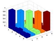 | 0.188 | 0.108 | |
4.4. Layout comparative analysis
Table 4 shows the layout of the five measuring points screened by EIM, KEM, and stepwise addition method based on QR decomposition and the stepwise subtraction method based on QR decomposition.
Table 4 intuitively shows the layout of measuring points screened by different methods. It can be seen from that in terms of uniformity of measuring points layout, QR- > QR+> EIM > KEM. Such result further verified the accuracy of the results specified in Table 3. Therefore, by observing the uniformity of measuring points layout, the superiority of the layout schemes could be assessed to a certain extent.
4.5. Optimal number of sensors
The above series of analyses were carried out based on the application of 5 measuring, but variation in the number of measuring points would also affect the optimization effect. In this section, the optimal number of sensors was selected by increasing the number of sensors one by one.
Table 4Measuring point layout of four optimization methods
Node number | 1 | 2 | 3 | 4 | 5 | 6 | 7 | 8 | 9 | 10 | 11 | 12 | 13 | 14 | 15 | 16 | 17 | 18 | 19 | 20 | 21 | 22 | 23 | 24 | 25 | 26 | 27 | 28 | 29 | 30 | 31 | 32 | 33 | 34 | 35 |
Element division |  | ||||||||||||||||||||||||||||||||||
EIM | ■ | ■ | ■ | ■ | ■ | ||||||||||||||||||||||||||||||
KEM | ■ | ■ | ■ | ■ | ■ | ||||||||||||||||||||||||||||||
Stepwise addition of QR decomposition | ■ | ■ | ■ | ■ | ■ | ||||||||||||||||||||||||||||||
Stepwise subtraction of QR decomposition | ■ | ■ | ■ | ■ | ■ | ||||||||||||||||||||||||||||||
Note | ■ means that the sensors arranged on the node | ||||||||||||||||||||||||||||||||||
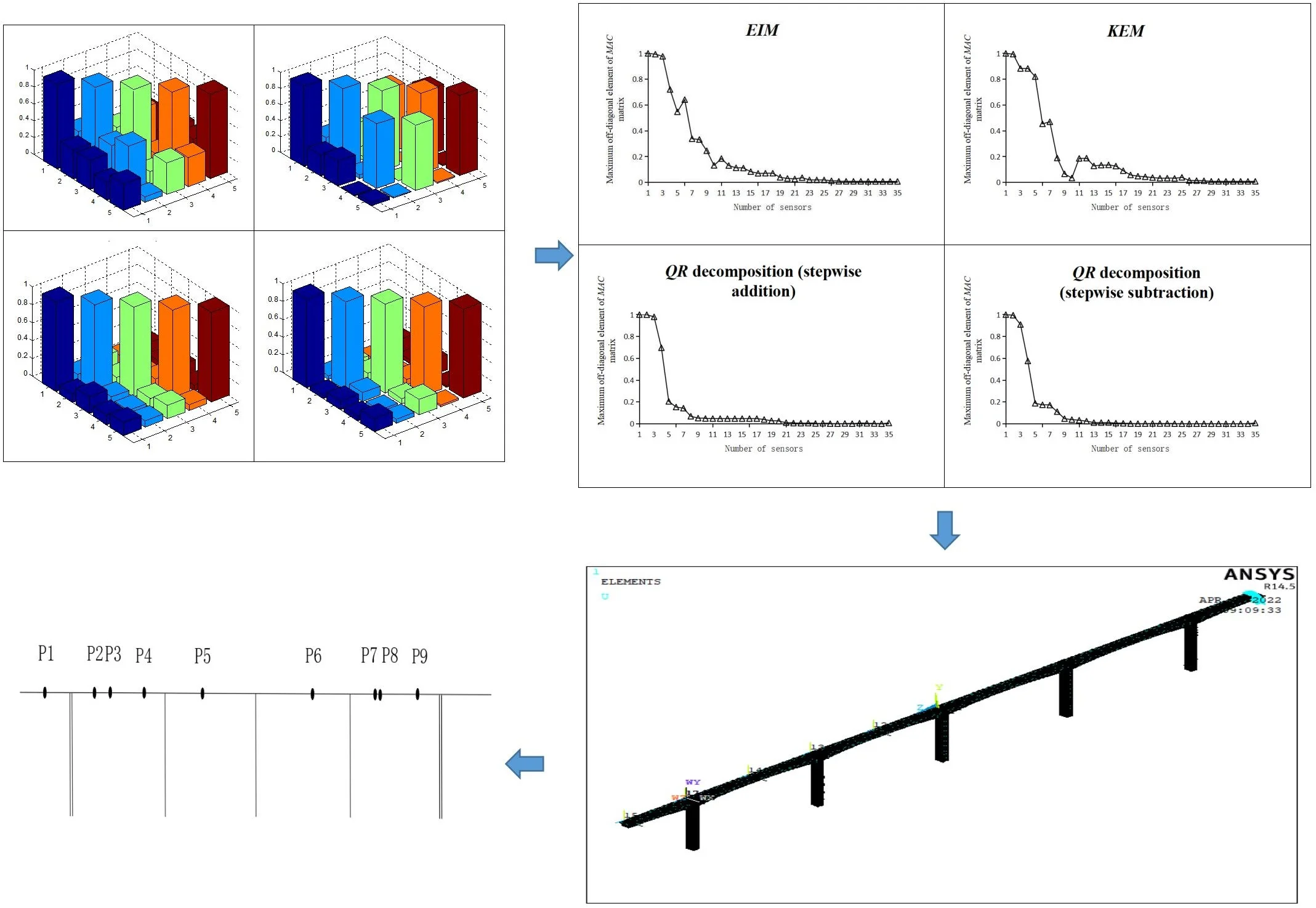
Figs. 3(a-d) show the comparison of the maximum off-diagonal element values of the MAC matrix and the change trend in the number of sensors obtained by using EIM, KEM, stepwise addition method based on QR decomposition and stepwise subtraction method based on QR decomposition.
Fig. 3Curve of maximum off-diagonal element of MAC and number of sensors
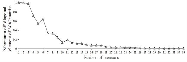
a) EIM
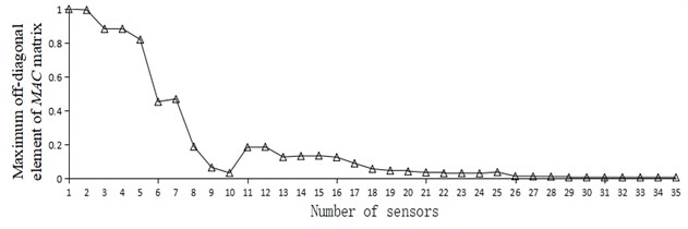
b) KEM
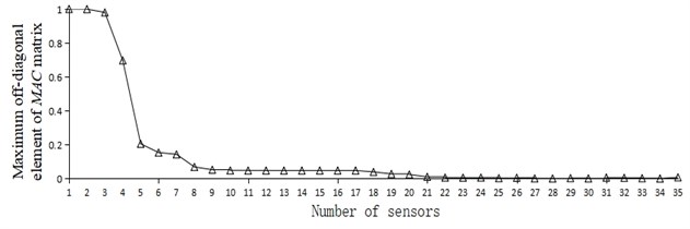
c) Stepwise addition of QR decomposition
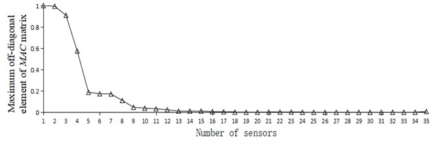
d) Stepwise subtraction of QR
It can be seen from Fig. 3 that no matter which layout scheme was adopted, with the increase of the number of sensors deployed on the measuring point, the maximum off-diagonal element of the MAC matrix showed a decreasing trend. By observing Fig. 3(a-d), it is apparent that the corresponding ordinate data in Fig. 3(c) and 3(d) declined significantly earlier than in Fig. 3(a) and 3(b), indicating that the method based on QR decomposition had better optimization foundation.
According to the research of relevant scholars [25], when the Modal Assurance Criterion was adopted for the optimal layout of measuring points, the maximum off-diagonal element value of MAC matrix was generally not greater than 0.25. Table 5 lists the number of sensors when the maximum off-diagonal element value was less than 0.25 and reached a very small steady state by different methods.
Table 5Comparison of MAC factor values of four optimization methods
Methods | EIM | KEM | Stepwise addition of QR decomposition | Stepwise subtraction of QR decomposition | ||||
Types | Number of sensors | Largest off-diagonal element value | Number of sensors | Largest off-diagonal element value | Number of sensors | Largest off-diagonal element value | Number of sensors | Largest off-diagonal element value |
Preset threshold of 0.25 | 9 | 0.245 | 8 | 0.189 | 5 | 0.205 | 5 | 0.188 |
Optimal sensor layout of various methods | 10 | 0.132 | 10 | 0.034 | 8 | 0.069 | 9 | 0.047 |
Comprehensive optimal sensor placement | Stepwise subtraction of QR decomposition | 9 | 0.047 | |||||
After comprehensive consideration of economic cost and test accuracy, the scheme adopted for the cantilever simply supported beam structure was determined as per the stepwise subtraction method based on QR decomposition. The number of sensors was set as 9, and the maximum off-diagonal element was 0.047.
5. Research on new method of optimal layout of measuring points
5.1. Background of proposed new method
It can be seen from the above theoretical analysis and numerical case that the MAC matrix composed of the modal information for the measuring points can reflect the state information of the whole structure. Therefore, this study is focused on how to screen out the appropriate number and layout of the sensors. Although the layout methods of EIM, KEM, QR+ and QR- could screen out a suitable number of measuring points for sensor layout, these methods were weak more or less in terms of over-reliance on the selection of initial measuring points, excessive number of measuring points and poor layout uniformity, and may not necessarily reflect the modal information of the complete structure, resulting in poor screening effect of measuring points. In view of this, an optimization method based on QR decomposition was proposed in this section.
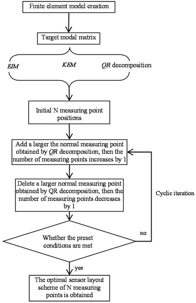
5.2. Number of sensors
The measuring point optimization layout method proposed in this section was mainly divided into two stages: the first stage was based on the conventional EIM, KEM and QR decomposition methods to select the initial measurement points. The second stage consisted in the replacement and adjustment based on the initial measuring point group. A larger normal measuring point obtained by QR decomposition was selected from the remaining measurement points and added to the selected measuring point group, and then a smaller normal measuring point obtained by QR decomposition was subtracted, and the number of measuring points remained unchanged. The cyclical iteration process, which took place until the optimal measuring point layout was obtained, is shown in Fig. 4.
Fig. 4Processing procedure as per optimal sensor layout method based on stepwise addition and subtraction of number of measuring points
5.3. Verification of numerical case as per new method
In order to verify the effectiveness of the proposed method and facilitate the comparison with conventional methods, 5 sensor measuring points were preset in this section. MATLAB software was used to compile the corresponding calculation program, and the results after stepwise addition and subtraction could be obtained as shown in Table 6.
Table 6MAC factor values and their variations for various stepwise addition and subtraction methods
Project | Initial layout scheme | Maximum off-diagonal element | Average off-diagonal element | Number of iterations | Largest off-diagonal element | Average off-diagonal element | Maximum off-diagonal element change | Average off-diagonal element change |
EIM-stepwise addition and subtraction | 6 23 29 34 35 | 0.547 | 1 | 6 10 23 29 34 | 0.164 | 0.051 | –70 % | –84 % |
KEM-stepwise addition and subtraction | 5 6 29 33 34 | 0.806 | 2 | 6 10 22 29 33 | 0.081 | 0.03 | –90 % | –87 % |
QR decomposition-based stepwise addition and subtraction | 6 13 24 29 35 | 0.205 | 3 | 6 11 24 29 33 | 0.025 | 0.006 | –88 % | –95 % |
Table 6 lists the screening results of the initial measuring points and the processing results after the stepwise addition and subtraction of measuring points one by one as per the EIM, KEM and QR decomposition method. Clearly, the optimization effect was greatly improved after the sensor addition and subtraction process.
If to compare the changes of the maximum off-diagonal element, the KEM stepwise addition and subtraction method had the best optimization effect, because the maximum off-diagonal element decreased from 0.806 to 0.081, and the efficiency increased to 90 %.
If to compare the changes of the average off-diagonal element, the consolidated stepwise addition and subtraction method based on QR decomposition had the best optimization effect, because the average off-diagonal element decreased from 0.118 to 0.006, and the efficiency increased to 95 %.
According to the relevant data listed in Table 6, a comprehensive comparative analysis of the above three methods of optimal measuring point layout revealed that the optimal measuring point layout obtained by the consolidated stepwise addition and subtraction method based on QR decomposition was the best since various adverse effects of the initial measuring point layout could be basically eliminated, and the optimal layout with five sensors could be obtained.
6. Practical engineering analysis
6.1. Project overview
A large-span prestressed concrete continuous rigid-frame bridge has a total length of 1170 meters and a span of 2×(62.5+4×115+62.5) meters. The ANSYS finite element software was used to model the bridge and analyze its load. The whole bridge was divided into 143420 elements and 224098 nodes. The main beam was made of C55 concrete, the elastic modulus 3.55×10⁴Pa, the pier column was made of C40 concrete, and the elastic modulus 3.25×10⁴Pa, Poisson’s ratio was 0.2, density was 2.55×10³kg/m3. The lateral and longitudinal constraints were simulated by COMBIN14 spring elements, and the beam end supports were consolidated by vertical constraints. The finite element model is shown in Fig. 5.
6.2. Optimal layout scheme
Fig. 6 shows the optimal layout scheme of the main beam obtained by using the EIM, KEM, stepwise addition method based on QR decomposition, stepwise subtraction method based on QR decomposition and consolidated stepwise addition and subtraction method based on QR decomposition with 9 sensors for this continuous rigid-frame bridge project.
Fig. 5Finite element model of concrete continuous rigid frame bridge
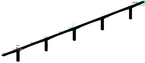
Fig. 6Comparison of layouts of different measuring point optimization schemes
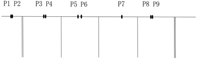
a) EIM
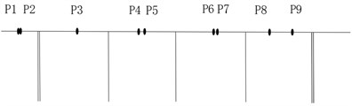
b) KEM
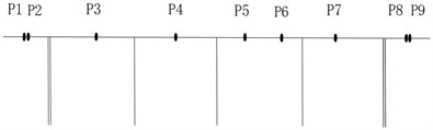
c) QR decomposition-stepwise addition
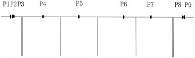
d) QR decomposition-stepwise subtraction
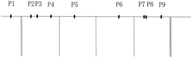
e) Consolidated QR decomposition-stepwise addition and subtraction
It can be seen from Fig. 6 that when the EIM or KEM was used, the layout of measuring points was more concentrated, because more measuring points were arranged in a concentrated area where the effective kinetic energy value was large. The basic idea of the method based on QR decomposition was to make the primary selection of measuring points based on a larger norm subset, so the position of the obtained measuring points will be more reasonable. Combined with the characteristics of the bridge type, the layout scheme of Fig. 6(d) using consolidated stepwise addition and subtraction method proposed in this study was adopted. Via this method, the measuring point positions were relatively uniform, and the layout density of the bridge spans such as side spans and middle spans were also considered. Therefore, the new method proposed was the most reasonable and can be used as a reference for the on-site sensor layout scheme.
Considering the actual engineering requirements, the number of measuring points was further expanded to 19. The layout scheme of measuring points for the main beam of continuous rigid frame bridge processed by the EIM, the KEM, stepwise addition method based on QR decomposition, stepwise subtraction method based on QR decomposition and consolidated stepwise addition and subtraction method based on QR decomposition is shown in Table 7.
Table 7 demonstrates that after the measuring points were optimized by the consolidated stepwise addition and subtraction method, the positions of the selected measuring points were more uniform, which could meet the actual monitoring requirements of the project.
Table 7Layout scheme of 19 measuring points with different methods
Method | Number of measuring points |
EIM | 8 9 10 11 41 42 43 44 75 76 77 78 116 117 147 148 149 150 151 |
KEM | 8 9 10 39 40 41 42 43 74 75 76 128 129 130 149 150 169 170 171 |
QR decomposition-stepwise addition | 9 10 23 42 55 57 58 77 87 102 110 121 134 149 165 169 177 182 183 |
QR decomposition-stepwise subtraction | 9 10 11 12 34 36 42 43 75 76 77 80 119 149 150 181 182 183 184 |
Consolidated QR decomposition-stepwise addition and subtraction | 4 10 28 34 37 48 70 83 97 101 112 113 127 131 146 146 173 182 184 |
7. Conclusions
In order to further improve the sensor optimization technology in bridge health monitoring, starting from the Modal Assurance Criterion and QR decomposition method, an optimal sensor layout method consisting in adding and subtracting the measuring points one by one cyclically was proposed, and it was verified in a sample of a simple cantilever beam and a continuous rigid frame bridge. The following conclusions can be drawn:
1) The smaller the off-diagonal element in the MAC matrix obtained based on the Modal Assurance Criterion is, the stronger the independence of the position of the structural measuring points will be, and the more accurately the real state of the structure can be reflected;
2) EIM, KEM, and stepwise addition method based on QR decomposition and stepwise subtraction method based on QR decomposition could optimize the number of sensors, but the optimization effect of EIM and KEM was poor when the number of measuring points was small. In addition, when the EIM was used for layout, only the modal information of each degree of freedom of the structure was considered, while the influence of some energy factors was ignored, resulting in poor layout stability.
3) The MAC matrix composed of modal information of finite measuring points can reflect the state information of the whole structure. Although the layout schemes of EIM, KEM, QR+ and QR- could optimize a suitable number of measuring points for the sensor layout, these methods are weak more or less in terms of over-reliance on the selection of initial measuring points, excessive number of measuring points and poor layout uniformity, and may not necessarily reflect the modal information of the complete structure, resulting in poor screening effect of measuring points.
4) This paper proposed an optimization and improvement method based on QR decomposition. By using EIM, KEM, QR decomposition method to filter the initial measurement points in order to obtain the processing results of stepwise adding and subtracting the measuring points one by one. Compared with conventional methods, the proposed method had the merit of greatly improving the layout effect and basically eliminating various adverse effects of the initial measuring point layout.
5) Relevant numerical case and engineering optimization examples could further prove that the application of the method proposed in this paper to optimize the measuring points could achieve higher uniformity of the selected measuring points, which could meet the monitoring requirements of actual projects.
References
-
Chen Yang, “Advances and prospects for optimal sensor placement of structural health monitoring,” Journal of Vibration and Shock, Vol. 39, No. 17, pp. 82–93, 2020.
-
G.-D. Zhou, T.-H. Yi, M.-X. Xie, H.-N. Li, and J.-H. Xu, “Optimal wireless sensor placement in structural health monitoring emphasizing information effectiveness and network performance,” Journal of Aerospace Engineering, Vol. 34, No. 2, p. 04020112, Mar. 2021, https://doi.org/10.1061/(asce)as.1943-5525.0001226
-
Bo Gao, Zhi-Hui Bo, and Yu-Bo Song, “Optimal placement of sensors in bridge monitoring based on an adaptive gravity search algorithm,” Journal of Vibration and Shock, Vol. 40, No. 6, pp. 87–92, 2021.
-
S. Desjardins and D. Lau, “dvances in intelligent long-term vibration-based structural health-monitoring systems for bridges,” Advances in Structural Engineering, Vol. 25, No. 7, pp. 1413–1430, 2022.
-
L.-M. Sun, Z.-Q. Shang, and Y. Xia, “Development and prospect of bridge structural health monitoring in the context of big data,” China Journal of Highway and Transport, Vol. 32, No. 11, Dec. 2019, https://doi.org/10.19721/j.cnki.1001-7372.2019.11.001
-
P. Rizzo and A. Enshaeian, “Bridge health monitoring in the United States: a review,” Structural Monitoring and Maintenance, Vol. 8, No. 1, pp. 1–50, 2021, https://doi.org/10.12989/smm.2021.8.1.001
-
A.-A. Zhang and X. Wu, “Optimal placement of bridge sensors based on IQPSO,” Computer Applications and Software, Vol. 38, No. 4, pp. 43–47, 2021.
-
J.-M. Li and Y.-F. Fu, “Analysis of improved algorithm of dynamic programming solving 0-1 knapsack problem,” Journal of Northwest University (Natural Science Edition), Vol. 44, No. 5, pp. 729–732, 2014.
-
B. Chen et al., “A hybrid method of optimal sensor placement for dynamic response monitoring of hydro-structures,” International Journal of Distributed Sensor Networks, Vol. 13, No. 5, 2017.
-
Yang Yang et al., “Optimal sensor placement for source tracking under synchronization offsets and sensor location errors with distance-dependent noises,” Signal Processing, Vol. 193, p. 108399, Nov. 2021, https://doi.org/10.1016/j.sigpro.2021.108399
-
W. Ostachowicz, R. Soman, and P. Malinowski, “Optimization of sensor placement for structural health monitoring: a review,” Structural Health Monitoring, Vol. 18, No. 3, pp. 963–988, May 2019, https://doi.org/10.1177/1475921719825601
-
D. C. Kammer, “Sensor placement for on-orbit modal identification and correlation of large space structures,” Journal of Guidance, Control and Dynamics, Vol. 14, No. 2, pp. 859–864, 1991.
-
J.-Z. Zhan and L. Yu, “An effective independence-improved modal strain energy method for optimal sensor placement,” Journal of Vibration and Shock, Vol. 36, No. 1, pp. 82–87, 2017.
-
P. Yu, M.-X. Chen, and K. Xie, “Optimal sensor placement for acoustic radiation prediction of cylinder shell based on proportion coefficient-effective independence method,” Journal of Ship Mechanics, Vol. 23, No. 5, pp. 621–629, 2019.
-
F. Sunca, F. Y. Okur, A. C. Altunişik, and V. Kahya, “Optimal sensor placement for laminated composite and steel cantilever beams by the effective independence method,” Structural Engineering International, Vol. 31, No. 1, pp. 85–92, Jan. 2021, https://doi.org/10.1080/10168664.2019.1704202
-
Ben-Israel A. and Greville T. N. E., “Generalized inverses,” in CMS Books in Mathematics, New York: Springer-Verlag, 2003, https://doi.org/10.1007/b97366
-
G. Heo and J. Jeon, “An experimental study of structural identification of bridges using the kinetic energy optimization technique and the direct matrix updating method,” Shock and Vibration, Vol. 2016, pp. 1–13, 2016, https://doi.org/10.1155/2016/3287976
-
Z.-C. Huang et al., “Damage identification of L-shaped pipeline based on modal strain energy change rate,” China Civil Engineering Journal, pp. 169–176, 2020.
-
G. Heo, M. L. Wang, and D. Satpathi, “Optimal transducer placement for health monitoring of long span bridge,” Soil Dynamics and Earthquake Engineering, Vol. 16, No. 7-8, pp. 495–502, May 1998, https://doi.org/10.1016/s0267-7261(97)00010-9
-
Y.-G. He, “Optimal sensors placement based on effective independence-entropy energy fusion method,” guangzhou, Guangzhou University, 2021.
-
X.-R. Qin and L.-M. Zhang, “Successive sensor placement for modal paring based-on QR-factorization,” Journal of Vibration, Measurement and Diagnosis, Vol. 21, No. 3, pp. 168–173, 2001.
-
H. Yin, “Optimal sensor placement and modal analysis of engineering structure,” Lanzhou, Lanzhou Jiaotong University, 2019.
-
X.-Q. Yin, X.-P. Liu, and G.-X. Wang, “Research progress of sensor optimization in high-rise building health monitoring,” Structural Engineers, Vol. 35, No. 2, pp. 220–225, 2019.
-
A.-M. Yuan, H. Dai, and Y.-H. Li, “Application comparison of optimization of sensor placement in modal test using EI method and MAC method,” Industrial Buildings, Vol. 38, pp. 343–347, 2008.
-
L.-B. Wang, Q.-L. Wang, Z. Zhu, and Y. Zhao, “Current Status and prospects of research on bridge health monitoring technology,” China Journal of Highway and Transport, Vol. 34, No. 12, p. 25, Feb. 2022, https://doi.org/10.19721/j.cnki.1001-7372.2021.12.003
Cited by
About this article

This work was partially supported by the Research Project of Jiangxi Provincial Department of Education (GJJ190980) and the Scientific Research Project of the Communications Department of Shaanxi Province (13-25k).
