A deformable derivative approach to Euler’s theorem for homogeneous functions and its extension to higher order partial derivatives

Naidu, Anju Dhiraj Kumar; Ahmad, Anisa; Ujlayan, Amit

doi:10.21595/mme.2026.25815

Mathematical Models in Engineering

Browse Journal

Submit article

Published: June 11, 2026

Check for updates

A deformable derivative approach to Euler’s theorem for homogeneous functions and its extension to higher order partial derivatives

Anju Dhiraj Kumar Naidu¹

Anisa Ahmad²

Amit Ujlayan³

^{1, 2}Department of Mathematics, G H Raisoni University, Amravati, Maharashtra, 444701, India

³Department of Applied Mathematics, School of Vocational Studies and Applied Sciences, Gautam Buddha University, Greater Noida, Uttar Pradesh, 201312, India

Corresponding Author:

Anju Dhiraj Kumar Naidu

Cite the article Download PDF

Article in Press

Downloads 19

Abstract

The deformable derivative is a recently proposed mathematical tool that interpolates between a function and its classical derivative using a parameterized limit. Initially introduced for single-variable functions, the concept is inherently fractional and has shown promise in various analytical applications. While fractional calculus is a fundamental tool for modeling non-linear, non-local and memory-based systems, it lacks the algebraic simplicity of higher-order derivatives when applied to multivariate calculus. To address this gap, a significant extension of the deformable derivative to multivariable functions is introduced by defining partial deformable derivatives in each coordinate direction while maintaining analytic consistency with classical calculus, and the validation is conducted through several test functions. To further address the lack of higher-order generalizations, the formulation is extended to include second-order deformable derivatives, yielding a higher-order Euler-type theorem. Unlike fractional calculus that relies on complex kernel, the novel method provides a local, computationally efficient identity that preserves the structural elegance of classical homogeneity. Several examples are provided to demonstrate the theoretical results and confirm the smooth convergence of the deformable Euler theorem to its classical counterpart. The proposed framework offers new tools for analysing homogeneous functions and provides a foundation for further extensions in partial differential equations and geometric analysis.

A deformable derivative approach to Euler’s theorem for homogeneous functions and its extension to higher order partial derivatives

Highlights

The deformable derivatives are extended to multivariable functions with partial deformable derivatives in each coordinate direction, preserving analytical consistency with classical calculus.
A novel Euler-type theorem for homogeneous functions is developed with partial deformable derivatives and by adding a tuning parameter to smoothly transition between function scaling and differential behavior.
The second-order deformable derivative formulation is then extended, producing a higher-order Euler identity that consolidates curvature and gradient effects in a consistent local manner.

1. Introduction

The deformable derivative is a brand-new idea in fractional calculus, which provides a nice smooth interpolation between a function and the classical derivative of a function via a differential form that has a parameter. The fractional calculus is particularly useful for modeling systems that exhibit non-local behaviours or memory-based features, its ability to capture memory, nonlinearity, and fractional behaviours makes it a fundamental tool. Since fractional calculus is a direct generalization of classical calculus, it does not include integer order derivatives and its extension to higher order partial derivatives.

The deformable derivative is developed to overcome the shortcoming of conformable derivative which lacks to include zero and negative numbers. Unlike a traditional fractional derivative, which is traditionally defined using integral operators, the deformable derivative is based entirely on limits, and this is helpful for symbolic manipulation and local analysis. The deformable derivative allows for a blending of functional value and rate of change (derivative), meaning that the operator allows for some flexibility, and is more appropriate for mapping intermediate behaviours within dynamical systems. The deformable derivative is popular for its simplicity, analytical tractability, and compatibility with classical differential operators. Another important characteristic is that it provides a parameter-based generalization of the derivative that can be modified to model systems, with behaviour that is varying in time, or memory-based behaviour, in a simple or antique way. Consequently, this operator has gained the interest of researchers seeking simplified variants of classical fractional models in mathematics and applied sciences. Despite its first promise, however, the theoretical background underlying deformable derivatives is relatively undeveloped, especially in multivariable contexts which interest real-world applications [1-4].

Most current literature on deformable derivatives focuses only on single-variable functions and fails to reframe the analysis in a multivariable approach. This limitation narrows the application of deformable derivatives for systems with spatial gradients, multi-parameter situations, or couplings with different differential equations. In addition, classical results of multivariable importance (such as Euler's theorem for homogeneous functions) have not been restated in a deformable form. The lack of a formal definition and structural inclusion, for partial deformable derivatives as presented in multivariable identities restricts exploring scale-invariance and fractional homogeneity. Furthermore, there is no set of higher-order models to represent curvature, diffusion, and second-order effects in deformable media as called for. Even though deformable derivatives are promising approaches, the current state of knowledge offers limited information and does not yet provide a complete and viable form to replace traditional multivariable differential approaches [5-8].

Many papers evaluated generalized fractional derivatives of multi-variable functions using integral-based operators like Riemann-Liouville or Caputo versions. These operators are useful; however, these types of formulations tend to be nonlocal with no simple differential structure, which makes them difficult to manipulate symbolically and extend classical identities. While the deformable derivative has an entirely limit-based formulation, considering a deformable partial derivative (DPD) along with methods that can connect deformable derivatives and classical multi-variable theorems like Euler's identity for homogeneous functions has yet to be presented. The majority of the literature on this topic is numerical approximations, discrete approximations, or limits that do not extend to multi-variable functions. The literature on deformable derivatives does not account for the higher-order formulations that are required to model curvature, expansion, or second-order dynamical systems [9-12].

Furthermore, the majority of existing research on deformable derivatives only focused on numerical approximation, discrete applications or limit-based definitions without extending to high-dimensional multivariable functions and does not account for high-order formulations. These gaps highlight the need for an advanced framework that extends to multivariable settings and supports higher-order formulations. Thus, the major contribution of the research is as follows:

1) To address the algebraic simplicity of higher-order derivatives in multivariate calculus, the deformable derivative is extended to the multivariable functions, which ensures analytical consistency with classical calculus thus enabling a unified treatment of function and derivative behavior.

2) To emphasize higher-order generalizations, second-order deformable derivatives are incorporated in the framework to obtain a higher-order Euler-type theorem, which helps to maintain analytical consistency with classical results, thereby enhancing multivariable analysis.

2. Literature survey

This section examines the development of earlier methods and their mathematical formulations, and discusses their strength and limitations to identify existing research gaps.

Al-Sharif et al [13] utilized fractional-order Chelyshkov functions (FCHFs) and their properties, and developed numerical method to solve multi-term variable-order fractional differential equations. Also, derived operational matrix of variable-order fractional integral for FCHFs, and reduced the computational effort required to approximate solutions of multi-term variable-order fractional differential equations where the variable-order fractional derivative and the variable-order fractional integral are considered in the Caputo sense and the Riemann-Liouville sense. This model further used fractional-order basis functions and provided different options to obtain either the exact solutions or accurate approximate solutions. This model reduced computational effort required to approximate solutions of multi-term variable-order fractional differential equations, but does not account for the higher-order formulations.

Khodabandehlo [14] introduced computational methods based on Bernoulli operational matrix (NBOM) for the generalized non-linear multi-term variable-order fractional differential equations. This model presented the fractional derivatives of Caputo, produced Bernoulli polynomials in estimating any unknown arbitrary function, approximated the function using Bernoulli polynomials, transformed the original problem into a set of algebraic equations that were solved using numerical techniques in collocation points, and finally implemented on several nonlinear multi-term variable-order fractional differential equations and evaluated. This model yielded high-accuracy approximate solutions even with a limited number of basic functions. However, when applied to multivariable functions and high-dimensional problems, it faces several limitations, primarily related to computational complexity and constraints on the domain.

Postavaru et al. [15] introduced the concept of fractional hybrid functions formed by block-pulses and fractional Fibonacci polynomials, and defined an exact integral operator. Moreover, derived the fractional nature of the operator through the $x \to x α$ transformation. The model used the regularized beta function, constructed integral operator from a technical standpoint and applied this operator to collocate the equations at the Newton-Cotes nodes. Further, this model applied this operator and collocated the equations at the Newton-Cotes nodes to reduce the multiterm fractional variable-order differential equation to a system of algebraic equations, which was then solved using Newton’s iterative method. This model focused on fractional derivatives in the Caputo sense and fractional integrals in the Riemann-Liouville sense, and solved multiterm variable-order fractional differential equations. Moreover, this model simplified for real-world applications, where computational resources are often limited, but high accuracy is still required.

Kostić [16] introduced and analyzed several types of fractional partial difference operators using the multidimensional convolution product. Here, this model discussed some classes of the fractional partial differential-difference with Riemann-Liouville and Caputo Derivatives, and solved multiterm fractional partial differential equations with Riemann-Liouville and Caputo Derivatives and fractional partial difference equations with generalized Weyl Derivatives, and established the complex characterization theorem for the multidimensional vector-valued Laplace transform and provided certain applications. Even though it analyzed several new types of fractional partial difference operators, this model lacks to accurately model complex, anisotropic, or non-homogeneous media in higher dimensions.

Zayed et al. [17] introduced and systematically developed a new class of hybrid multidimensional polynomials, and constructed through a convolution of Frobenius-Euler and multivariate Hermite polynomials. Moreover, this model conducted computational simulations to visualize and analyze the distribution of polynomial zeros, providing empirical validation of their structural properties, and the approximated roots exhibited symmetry and regularity patterns consistent with the theoretical framework. This model also discussed the polynomials under parameter variation, especially in high-dimensional settings, and established a foundational analytical framework for multivariate Hermite-Frobenius-Euler polynomials. This model lacks to investigate their symmetry properties, and determinantal structures, and does not contribute to advancements in both analytical theory and computational implementation.

Nilsson et al. [18] discussed optimization of functions without Lipschitz continuous gradients by leveraging the concept of relative smoothness, with respect to a reference function. This model derived calculus rules for the symmetry coefficient, and computed $α$ ( $∥ \cdot ∥ p 2$ ) for general $p$ . Moreover, this model established upper and lower bounds for the symmetry coefficient of sums of positively homogeneous Legendre functions, and provided exact formulas for these sums, under certain conditions. Also, provided closed-form computations for specific cases such as $p \in$ {6, 8, 10}. This model directly related symmetry coefficient of a positively homogeneous, Legendre functions to the degree of homogeneity and the structure of its derivatives, with significant limitations arising when examining higher-order properties.

Alawaideh, et al. [19] investigated two systems using the conformable version of the calculus of variations to derive the fractional Euler-Lagrange equation. This model applied this calculus to the conformable version of classical mechanics, introduced the conformable Lagrangian and derived the equation of motion. Moreover, the obtained path integral quantization directly as an integration over the canonical coordinate without the need of integration over the variable. This model discussed nonlinear dynamics and invariance principles in complex systems involving controlled Lagrangians with higher-order derivative. Moreover, this model demonstrated invariance results concerning state variables and explored a natural Hamiltonian formulation for composite higher derivative theories involving time derivatives using enhanced theoretical applications in this domain, without expanding research on conformable derivatives and generalized point particles advancing the understanding of these complex systems.

Godinho et al [20] introduced the Riemann-Liouville, Gerasimov-Caputo, Grünwald-Letnikov, and Riesz formulations, and presented fractionality-inspired conformable derivative as an alternative approach to local calculus that maintains the Leibniz rule while introducing scale-dependent dynamics and a fractional parameter. This model included the fractional Laplacian and its connection to the Riesz derivative, and intimately related the conformable calculus to the fractal calculus. Moreover, this model discussed Fractional Action-Like Variational Approach (FALVA) for introducing non-locality and memory effects into the action principle rather than the equations of motion. This model lacks the fractional calculus since it continues to evolve as a rich mathematical theory in continuous construction in its multiple manifestations, and with a growing number of applications across all physical scales.

Youssri et al. [21] introduced a Petrov-Galerkin method (PGM) to address the fourth-order uniform Euler-Bernoulli pinned-pinned beam equation. Utilizing a suitable combination of second-kind Chebyshev polynomials as a basis in spatial variables, this model elegantly and simultaneously satisfied pinned-pinned and clamped-clamped boundary conditions. Moreover, derived explicit formulas for the inner product between these basis functions and their derivatives with second-kind Chebyshev polynomials, which leads to a simplified system of algebraic equations with a recognizable pattern. Furthermore, provided inversion to an approximate spectral solution. The efficiency of this model described in precisely solving the Euler-Bernoulli beam equation under different scenarios has been validated by numerical testing, meanwhile, it increased complexity in selection.

These limitations highlight a clear research gap, which motivates the present study. Accordingly, this framework develops a generalized deformable derivative framework for multivariable functions and proposes a novel extension to Euler’s theorem, along with its higher-order formulations.

3. Proposed methodology

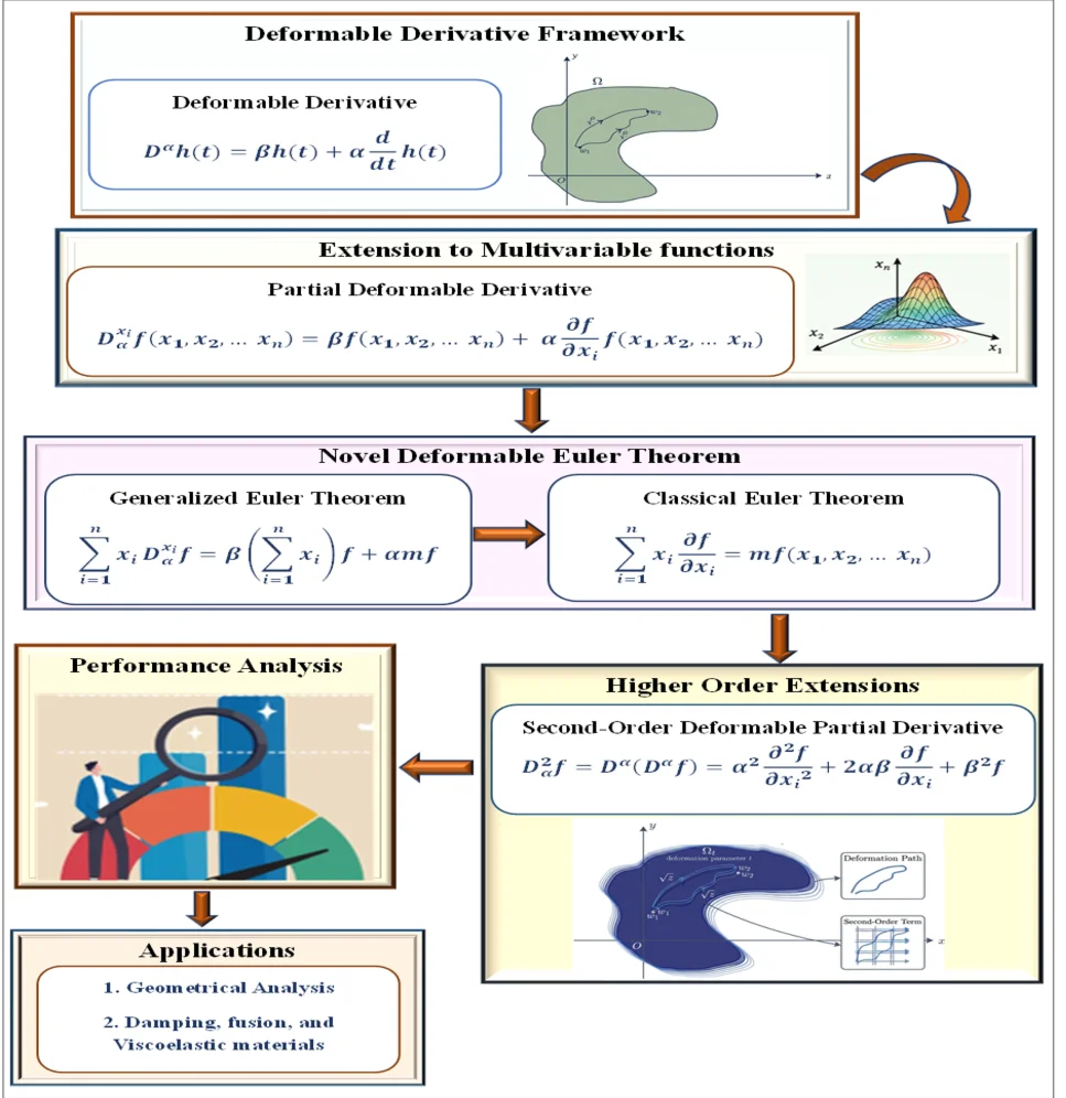
The concept of the deformable derivative is extended to multivariable functions to address the limitations of its existing formulation, which is primarily restricted to single-variable analysis and does not adequately handle functions involving multiple variables. This extension utilizes the linear structure of the deformable derivative and serves as a smooth generalization of classical results. Furthermore, this framework introduces a higher-order extension of this new version of Euler’s theorem via deformable partial derivatives.

3.1. Deformable derivatives and their properties: a basic definition

This section focuses on extending the concept of the deformable derivative to multivariable functions. Unlike existing fractional derivative, which primarily emphasize nonlocality and memory effects, the deformable derivative incorporates a single deformable parameter that blends the function value and its derivative into a unified analytical expression. This formulation preserves consistency with classical calculus while introducing a flexible parameter that enables smooth interpolation between the function and its derivative behavior

3.1.1. Definition 3.1.1 (deformable derivative)

Many modeling systems often involve dynamic behavior and memory effects that classical derivatives alone cannot capture, such as damping in materials, energy dissipation, or non-local stress-strain relationships. The deformable derivative is a hybrid mathematical operator that provides a smooth, linear interpolation between a function and its classical first-order derivative, allowing the modeling system to model the dynamic behavior and memory effects in a flexible and tunable way.

Let $h (t)$ be a function with a real value that is defined on the open interval $(a, b) .$ For any real parameter $α \in [0,1]$ , the deformable derivative of $h$ at $t$ , denoted by $D^{α} h (t)$ , is defined as Eq. (1) [22]:

1

D^{α} h (t) = \begin{matrix} l i m \\ e \to 0 \end{matrix} \frac{(1 + ε β) h (t + α ε) - h (t)}{ϵ},

where $β = 1 - α$ . If this limit exists, then $h$ is said to be $α$ -differentiable at $t$ , and $D^{α} h (t)$ denotes its deformable (or fractional) derivative.

3.1.2. Remark 3.1.2

The definition is consistent with classical differentiation in two extreme cases:

– If $α = 0$ , then $D^{0} h (t) = h (t)$ , i.e., the deformable derivative returns the function itself.

– If $α = 1$ , then $D^{1} h (t) = h (t)$ , the classical (first-order) derivative.

Thus, the deformable derivative provides a smooth interpolation between the function and its classical derivative, and is sometimes referred to as the $α$ -derivative.

3.1.3. Theorem 3.1.3 (continuity from deformability)

If $h (t)$ is $α$ -differentiable at a point $t_{0} \in (a, b)$ for some $α \in (0,1]$ , then $h$ is continuous at $t_{0}$ .

Proof sketch:

Since $D^{α} h (t)$ exists, the limit in Definition 3.1.1 exists, and the limit expression ensures continuity in the classical sense. This mirrors the logic used in classical analysis.

3.1.4. Theorem 3.1.4 (properties of deformable derivative)

Let $h_{1} (t)$ and $h_{2} (t)$ be $α$ – differentiable at $t$ be a basis functions, $t$ be an independent variable, $a$ and $b$ be a constants, and $β$ be a scaling parameter or eigenvalue that relates the constant to its own fractional derivative, then the deformable derivative operator $D^{α}$ satisfies the following properties:

(a) Linearity: $D^{α} [a h_{1} (t) + b h_{2} (t)] = a D^{α} h_{1} (t) + b D^{α} h_{2} (t),$ for all $a, b ϵ R$ .

(b) Commutativity: $D^{α_{1}} (D^{α_{2}} h (t)) = D^{α_{2}} (D^{α_{1}} h (t))$ .

(c) Constant Function Rule: $D^{α} s = β s$ , for any constant $s \in R$ .

(d) Product Rule (Modified): $D^{α} [h_{1} (t) \cdot h_{2} (t)] = (D^{α} h_{1} (t)) \cdot h_{2} (t) + α h_{1} (t) \cdot \frac{d}{d t} h_{2} (t)$ , where, $h_{1} (t)$ and $h_{2} (t)$ is a basis functions, $t$ is independent variable, $a$ and $b$ is constants, $β$ is scaling parameter or eigenvalue that relates the constant to its own fractional derivative, and $D^{α}$ is deformable derivative operator.

Thus, Leibniz’s rule does not hold exactly; this deviation reinforces the interpretation of $D^{α}$ as a fractional-type operator.

(e) Function-Derivative Linear Relation:

The function-derivative linear relation is defined by the following Eq. (2) [23] to show that the last identity is particularly significant to show how the deformable derivative is linearly dependent on both the function and its classical derivative:

2

D^{α} h (t) = β h (t) + α \frac{d}{d t} h (t),

where, $α \frac{d}{d t} h (t)$ is the first-order derivative, and this formulation provides a flexible framework that smoothly interpolates between purely functional and purely differential behaviour. Thus, the proposed approach provides a foundational framework for multivariable analysis, ensuring smooth compatibility with classical results and facilitating further developments such as higher-order generalizations and deformable extensions of fundamental theorems.

3.2. Deformable derivative for multivariable functions and a new form of Euler’s theorem

This section presents a generalized form of Euler’s theorem for homogeneous functions using Deformable Partial Derivatives (DPDs) by extending the formulation to second-order deformable derivatives, yielding a higher-order Euler-type theorem that generalizes classical results and enhances the analysis of multivariable homogeneous functions.

3.2.1. Extension to multivariable functions

The deformable partial derivative of a multivariable function denoted as $D_{α}^{x_{i}} f$ is a local, limit-based operator designed to provide a smooth interpolation between a function’s value and its classical rate of change.

Let $f (x_{1}, x_{2}, \dots x_{n})$ be a real-valued function defined on an open subset of $R^{n}$ and $α \frac{\partial f}{\partial x_{i}}$ be a non-linear term. Then define the partial deformable derivative of $f$ to the variable $x_{i}$ , denoted by $D_{α}^{x_{i}} f$ , as Eq. (3) [24]:

3

D_{α}^{x_{i}} f (x_{1}, x_{2}, \dots x_{n}) = β f (x_{1}, x_{2}, \dots x_{n}) + α \frac{\partial f}{\partial x_{i}} f (x_{1}, x_{2}, \dots x_{n}),

where, $f (x_{1}, x_{2}, \dots x_{n})$ is real-valued function defined on open subset of $R^{n}$ , $α \frac{\partial f}{\partial x_{i}}$ is non-linear term, and $β = 1 - α$ , this formulation establishes a consistent extension of the deformable derivative to multivariable functions by defining the operator along each coordinate direction. It preserves the linear relationship between the function and its first-order partial derivates, ensuring compatibility with classical calculus while enabling a smooth transition toward generalized behavior. As a result, the deformable partial derivative provides a unified and flexible analytical framework for studying multivariable functions.

3.2.2. Novel Euler’s theorem using the deformable derivative

Recall that a function $f (x_{1}, x_{2}, \dots, x_{n})$ is said to be homogeneous of degree $m$ if for any scalar $λ > 0$ : $f (λ x_{1}, λ x_{2}, \dots, λ x_{n}) = λ^{m} f (x_{1}, x_{2}, \dots, x_{n})$ , where $λ$ is a scaling factor.

By relating the parameters including the elasticity of the function $m$ , and the sum of the coordinate positions $\sum_{i = 1}^{n} x_{i}$ , the classical Euler’s theorem is defined as $\sum_{i = 1}^{n} x_{i} \frac{\partial f}{\partial x_{i}} = m f (x_{1}, x_{2}, \dots x_{n})$ .

Now propose the novel deformable Euler’s theorem, using definition of the partial deformable derivative in Eq. (4):

4

\sum_{i = 1}^{n} x_{i} D_{α}^{x_{i}} f = \sum_{i = 1}^{n} x_{i} (β f + α \frac{\partial f}{\partial x_{i}}) = β (\sum_{i = 1}^{n} x_{i}) f + α \sum_{i = 1}^{n} x_{i} \frac{\partial f}{\partial x_{i}} .

Since $f$ is homogeneous of degree $m$ , use the classical Euler result [25]:

5

\sum_{i = 1}^{n} x_{i} \frac{\partial f}{\partial x_{i}} = m f .

The novel deformable Euler’s Theorem for homogeneous functions defined by substituting the classical Euler result in function of homogeneous of degree $m$ in Eq. (4) given by Eq. (5) [25] as:

6

\sum_{i = 1}^{n} x_{i} D_{α}^{x_{i}} f = β (\sum_{i = 1}^{n} x_{i}) f + α m f .

The Eq. (6) demonstrates how the contribution of the function $f$ and its partial derivatives are blended using the deformation parameter $α$ , offering a smooth transition from the function’s scaled value to its differential structure. Thus, the deformable parameter $α$ allows the modeling system to interpolate pure scaling behaviour and the derivative effects, while the scaling factor $β$ introduces an additional flexibility that allows the modeling of the non-uniform materials, fractional structures or imperfect homogeneity.

3.2.3. Extension to higher-order partial deformable derivatives

The higher-order deformable partial derivatives are calculated by applying the DPD operator multiple times through sequential deformation. The higher-order partial deformable derivatives obtained by extending Euler’s Theorem for homogeneous function lies in the limitation of classical calculus to describe anisotropic and non-local growth. The higher-order partial deformable derivatives function contains the classical theory as a singular, ideal point.

By blending the function value $f$ , first-order gradient $\frac{\partial f}{\partial x_{i}}$ and second-order partial derivative $\frac{\partial^{2} f}{\partial {x_{i}}^{2}}$ , the second-order deformable operator $D_{α}^{2} f$ is defined by Eq. (7) [26]:

7

D_{α}^{2} f = D^{α} (D^{α} f) = α^{2} \frac{\partial^{2} f}{\partial {x_{i}}^{2}} + 2 α β \frac{\partial f}{\partial x_{i}} + β^{2} f .

Second-Order Euler-Type Identity.

Using (7) to bridge this with classical theory, a second-order Euler-type expression for a homogeneous function of degree is defined by Eq. (8):

8

\sum_{i = 1}^{n} {x_{i}}^{2} D_{α}^{{x_{i}}^{2}} f + \sum_{i = 1}^{n} x_{i} D_{α}^{x_{i}} f = \sum_{i = 1}^{n} [{x_{i}}^{2} (α^{2} \frac{\partial^{2} f}{\partial {x_{i}}^{2}} + 2 α β \frac{\partial f}{\partial x_{i}} + β^{2} f) + x_{i} (β f + α \frac{\partial f}{\partial x_{i}})] .

This extended form blends contributions from function value $f$ , first-order gradient $\frac{\partial f}{\partial x_{i}}$ , and second-order partial derivative $\frac{\partial^{2} f}{\partial {x_{i}}^{2}}$ , and are used to derive higher-order generalizations of Euler’s identity within the deformable framework. By integrating function value, gradient and curvature into a single deformable framework, the proposed approach provides a more flexible analytical structure than classical calculus. Consequently, it serves as a flexible tool for modeling system where higher-order interactions are significant.

Remarks on the novel formulation.

1) By introducing a scaling bias, the proposed deformable Euler theorem provides a significant extension to classical calculus via $\sum x_{i}$ , which is absent in the classical formulation. This additional component enables the model to incorporate both the local value of the function and its rate of change, extending the applicability of Euler’s theorem beyond purely differential behaviour.

2) The formulation maintains mathematical integrity by ensuring that, in the limiting case $α = 1$ , it reduces exactly to the classical Euler’s theorem for homogenous functions. This limiting behaviour confirms that the proposed model is a consistent generalization of the classical result rather than an alternative formulation.

3) Furthermore, the introduction of the deformable parameter α provides a controllable mechanism to interpolate between the functional scaling and differential structures. This representation enhances the flexibility of the framework and allows it to be adapted for analytical and computational settings where a combined representation of state and rate-dependent behaviour is required.

4) The proposed model is particularly valuable for symbolic computing and generating approximate solutions in complex dynamical systems, especially where a mixed behaviour between the identity operator and the derivative is required to model real-world phenomena accurately.

Example. Let f $(x, y) = x^{2} + y^{2}$ , which is homogeneous of degree 2.

Classical Euler’s theorem: $x \frac{\partial f}{\partial x} + y \frac{\partial f}{\partial y} = 2 (x^{2} + y^{2})$ .

Deformable Euler’s theorem: $x D_{α}^{x} f + y D_{α}^{y} f = β (x + y) (x^{2} + y^{2}) + 2 α (x^{2} + y^{2})$ .

This result verifies the proposed deformable Euler’s theorem for a homogenous function of degree 2. The obtained expression includes an additional term involving the deformation parameter which represents a controlled deviation from the classical Euler identity and accounts for the contribution of the function value itself. The presence of the parameter $α \in [0,1]$ enables a controlled smooth transition between the function and its derivative for combining both scaling behaviour and differential structures within a unified framework. Furthermore, the additional term involving $β (x + y) (x^{2} + y^{2})$ introduces a flexible scaling component which is absent in the classical case. As a result, the proposed formulation extends the classical identity into a more adaptable analytical form, and allows a meaningful interpretation even when strict homogeneity conditions are relaxed, providing a more adaptable analytical tool. Overall, the proposed deformable Euler’s theorem is regarded as a generalized identity that bridges purely algebraic scaling and differential behaviour, offering a broader perspective than the classical formulation.

4. Applications and examples of deformable Euler’s theorem

This section demonstrates the applicability of the novel deformable Euler's theorem for homogeneous functions of multiple variables. The deformable Euler theorem for higher-order extensions is used effectively for modeling systems where traditional linear scaling and homogeneity do not apply. By deforming the derivative and by representing $f (x)$ as displacement field in the damping material, the first order DPD models energy dissipation, second order DPD models stiffness curvature coupling, so that the modeling system accurately capture the memory effects and energy dissipation in polymers or high-damping alloy that ignores standard calculus. Since these materials exhibit fractal-like properties and non-uniform density, the deformable Euler theorem forms an accurate relationship between the internal stress distribution and the total potential energy of the structure.

Using specific examples, the deformable Euler's theorem validates the correctness of the deformable formulation and explores how it generalizes classical Euler identities. The results further highlight how this approach interpolates between function scaling and classical differentiation using the deformability parameter $α \in [0,1]$ .

4.1. Example 1: homogeneous function of degree 2

The proposed formulation is validated through analytical examples to demonstrate its consistency with classical results and its generalized behaviour.

Let $f (x, y) = x^{2} + y^{2}$ .

Where $f$ is homogeneous of degree $m = 2$ .

(a) Classical Euler’s Theorem: $x \frac{\partial f}{\partial x} + y \frac{\partial f}{\partial y} = 2 (x^{2} + y^{2})$ .

(b) Deformable Eulers Theorem:

Compute the partial deformable derivatives:

D_{α}^{x} f = β f + α \frac{\partial f}{\partial x} = β (x^{2} + y^{2}) + α (2 x),

D_{α}^{y} f = β f + α \frac{\partial f}{\partial y} = β (x^{2} + y^{2}) + α (2 y) .

Now apply the deformable Euler identity:

{x D}_{α}^{x} f + y D_{α}^{y} f = x [β f + α (2 x)] + y [β f + α (2 y)] = β (x + y) (x^{2} + y^{2}) + 2 α (x^{2} + y^{2}) .

Thus, the deformable Euler result becomes:

{x D}_{α}^{x} f + y D_{α}^{y} f = [β (x + y) + 2 α] f (x, y) .

For $α = 1$ , $β = 0$ , this reduces to the classical identity.

4.2. Example 2: homogeneous function of degree 3

Let $f (x, y) = x^{3} + y^{3}$ .

Clearly, $f$ is homogeneous of degree $m = 3$ .

Compute:

\frac{\partial f}{\partial x} = 3 x^{2}, \frac{\partial f}{\partial y} = 3 y^{2},

D_{α}^{x} f = β f + α ∙ 3 x^{2}, D_{α}^{y} f = β f + α ∙ 3 y^{2} .

Now: ${x D}_{α}^{x} f + y D_{α}^{y} f = x (β f + 3 α x^{2}) + y (β f + 3 α y^{2}) = β (x + y) f + 3 α (x^{3} + y^{3})$ .

Hence: ${x D}_{α}^{x} f + y D_{α}^{y} f = β (x + y) f + 3 α (x^{3} + y^{3})$ .

This again confirms the proposed deformable Euler identity:

\sum_{i = 1}^{n} x_{i} D_{α}^{x_{i}} f = β (\sum x_{i}) f + α m f .

4.3. Example 3: second-order deformable derivative

Let us revisit $f (x, y) = x^{2} + y^{2} .$

For second-order deformable derivatives:

D_{α}^{2} f = α^{2} \frac{\partial^{2} f}{\partial x^{2}} + 2 α β \frac{\partial f}{\partial x} + β^{2} f .

Since:

\frac{\partial^{2} f}{\partial x^{2}} = 2, \frac{\partial f}{\partial x} = 2 x .

Then: $D_{α}^{{x_{i}}^{2}} f = α^{2} (2) + 2 α β (2 x) + β^{2} (x^{2} + y^{2})$ .

Similarly: $D_{α}^{{y_{i}}^{2}} f = α^{2} (2) + 2 α β (2 y) + β^{2} (x^{2} + y^{2})$ .

Using the proposed second-order Euler-like expression:

x^{2} D_{α}^{{x_{i}}^{2}} f + y^{2} D_{α}^{{y_{i}}^{2}} f + x D_{α}^{x} f + {y D}_{α}^{y} f = (x^{2} + y^{2}) [2 α^{2} + β^{2} (x^{2} + y^{2}) + β (x + y) + 2 α] + 4 α β (x^{3} + y^{3}) .

This completes the full symbolic expansion of the second-order deformable Euler-like expression for the function $f (x, y) = x^{2} + y^{2} .$

From the above examples, the first-order deformable derivative ( $D_{α}^{x_{i}} f = β f + α \frac{\partial f}{\partial x_{i}}$ ) models systems experiencing material aging or damping, providing a predictive scaling relationship though the identity $\sum_{i = 1}^{n} x_{i} D_{α}^{x_{i}} f = β (\sum_{i = 1}^{n} x_{i}) f + α m f$ , where the fractional calculus requires all time-steps or spatial points to evaluate a single derivative. The second-order deformable derivative enables formulation of generalized stiffness matrices by encoding the coupling between the displacement $f$ and curvature $\frac{\partial^{2} f}{\partial x^{2}}$ and validates finite element analysis (FEA) simulations.

4.4. Discussion and interpretation of results

The proposed deformable Euler theorem generalizes classical Euler’s identity when $α =$ 1, at this point, the operator $D^{α}$ collapses into standard second order derivative, and the deformable Euler theorem recovers the classical Euler theorem. The operator recovers the function itself ( $D^{0} f = f$ ), when $α = 0$ , which represents the zero-order state where the system’s derivation is purely proportional to its current magnitude. The deformable Euler theorem allows fractional-like intermediate behaviour when $α \in (0,1),$ and the parameter $α$ serves as a weighing factor which blends the function’s value with its derivate to account for non-local effects. Thus, the proposed framework models fractional like intermediate behaviour, blending functions and derivative, useful in non-local or memory dependant modeling phenomenon. Moreover, the proposed work encodes function-derivative coupling in a scalable form using a single parameter $α$ , and provides a consistent way to incorporate scaling bias and weighted differentiation in models with fractional dynamics. Furthermore, the deformable Euler theorem offers a unified mathematical framework for transitioning between classical and fractional regimes, and by employing a single parameter $α$ , it ensures consistency across different order of differentiation, making it an important tool for high-precision modeling in fractional calculus.

5. Results and discussion

The graphical results included in this section have been generated using python, based on the analytical expression derived in the proposed methodology, to illustrate the behaviour of the model under varying parameter conditions: Software Used: Python, OS: Windows 10 (64-bit), Processor: Inteli5, RAM: 16GB RAM.

5.1. Performance analysis of proposed model

This section offers a comprehensive analysis of the performance of the proposed model, based on the results obtained from the developed formula.

Fig. 1 shows the performance of the sensitivity of the system’s evolution with the change in the deformation parameter $α$ . As the value of $α$ increased from 0.25 to 0.75, the curve shifts upward and leftward, indicating that a higher differential weight causes the function to reach its saturation point much faster. This shows tuning $α$ acts as a speed controller for the scaling process. When all curves converge at $t = 4$ and $s (t) = 1$ , the final boundary state of the homogenous functions remains invariant. Thus, the flexibility of the deformable method on modeling different rates of scaling is increased without losing the underlying structure of original identity.

Fig. 2 illustrates the performance of the sensitivity of the system’s variable $x (t)$ over time $t$ under three different values of the deformation parameter $α$ . As the value of $α$ increases, the rate of the system increases, reaching higher magnitude at the end of the interval $t = 4$ . This indicates higher deformation parameter makes the parameter more sensitive to the scaling variable $t$ , which causes the homogeneous function to evolve more rapidly towards its upper limit. Conversely, a lower deformation parameter $α$ preserves more of the function’s initial stability, resulting in a flatter, more gradual transition.

Fig. 1Performance of sensitivity of system’s evolution with respect to change in deformation parameter

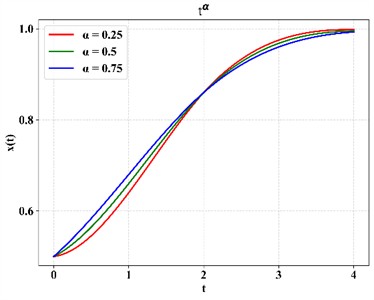
Fig. 2Performance of sensitivity of system’s variable over time

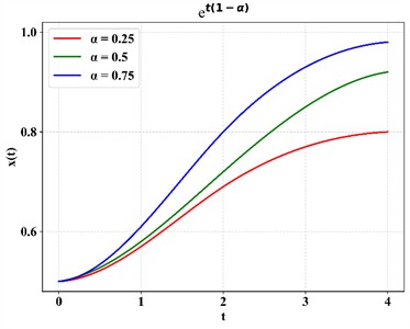
Fig. 3 illustrates the performance of the sensitivity of the functions $v (t)$ as it responds to the variation in the deformation parameter $α$ . As the value of $α$ increases from 0.25 to 0.75, the function exhibits a faster rate of growth and reaches its upper saturation point more quickly. A higher $α$ value makes the system more sensitive to the passage to the time $t$ , accelerating the transition. The convergence of all the three lines as they approach $t = 4$ demonstrates that while the deformation parameter $α$ alters the specific path and speed of the function’s development.

Fig. 3Performance of sensitivity of functions over time deformation parameter

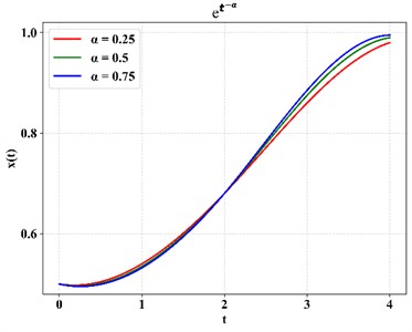
Fig. 4Performance of sensitivity of variable over deformation parameter

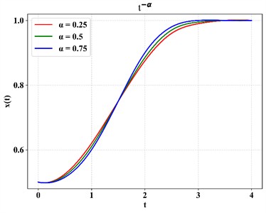
Fig. 4 illustrates the performance of the sensitivity of the variable $x (t)$ as it responds to the deformation parameter $α$ over a temporal scale. As the value of $α$ increases from 0.25 to 0.75, the system response becomes more non-linear. While a higher $α$ initially suppresses the function’s value, it eventually drives the system to its saturation points $(x (t) = 1)$ with greater velocity. This illustrates that in the deformable Euler method, $α$ controls the rate of convergence towards the homogenous limit, allowing the effective tuning of the system’s dynamic transition between its initial state and its steady state equilibrium.

5.2. Comparative analysis of proposed model with other models

This section provides a detailed explanation of the comparative analysis of the proposed model with other models based on achieved results.

Fig. 5 illustrates the comparative analysis of the deformation parameter $α$ in the deformable Euler Theorem with other methods. As the value of $α$ decreases through fractional Euler-Lagrange method (0.8) [27], fractional-order Chelyshkov collocation Method (0.25) [13] and fractional hybrid functions formed by block-pulses and fractional Fibonacci polynomials (1.0) [15], the operator becomes increasingly deformed. This suggests that the deformable Euler Theorem is designed to model system where the function’s local state is more influential than its curvature or steepness, providing stable generalization of Euler’s identity than traditional fractional method.

Fig. 5Comparative analysis of deformation parameter α in deformable Euler Theorem with other methods

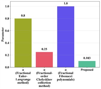
Fig. 6Comparative analysis of scaling parameter β in deformable Euler Theorem with other methods

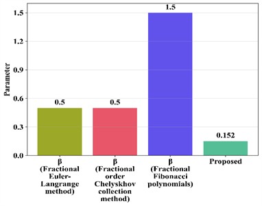
Fig. 6 illustrates the comparative analysis of the scaling parameter $β$ in the deformable Euler Theorem with other methods. The value of $β$ in the deformable Euler Theorem utilizes a smaller proportional value than other method including fractional Euler-Lagrange method (0.5) [27], fractional-order Chelyshkov collocation method (0.5) [13] and fractional hybrid functions formed by block-pulses and fractional Fibonacci polynomials (1.5) [15]. Within the deformable Euler Theorem, the low $β$ value allows to de-emphasize the functions’s magnitude $f$ , which effectively shifts the identity focus toward the deformation parameter $α$ . This suggests that the deformable Euler Theorem is designed to capture high-frequency variation and local curvature without the scaling bias present in fractional calculus.

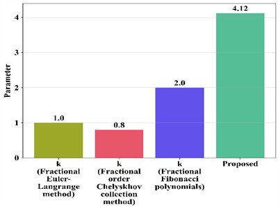
Fig. 7 illustrates the comparative analysis of the degree of homogeneity in the Deformable Euler Theorem with other method. The high $k$ value in the deformable Euler Theorem allows to handle higher-order non linearity. As the result of deformable Euler Theorem is directly proportional to the degree of homogeneity, a value of 4.12 indicates that the novel method can accurately model system that scale much more effectively than the fractional calculus.

Overall, the comparative analysis demonstrates that the proposed deformable Euler framework provides a more flexible and adaptable formulation than existing fractional methods. The deformation parameter $α$ enables controlled interpolation between function dominance and differential behaviour, while the scaling parameter $β$ allows selective emphasis on local variations. In contrast to traditional fractional approaches, the proposed model exhibits improved capability in capturing high-frequency variations and nonlinear scaling behaviour. Furthermore, its direct dependence on the degree of homogeneity enhances its effectiveness in modeling higher-order nonlinear systems. These characteristics confirms that the deformable Euler’s theorem offers a stable and generalized analytical framework with improved adaptability over existing methods.

Fig. 7Comparative analysis of degree of homogeneity in deformable Euler Theorem with other methods

6. Conclusions

The study presented a new extension of the deformable derivative to multivariable functions, where partial deformable derivatives were defined in each of the coordinate directions. Based on this framework, a generalized form of Euler’s theorem for homogeneous functions is developed in terms of deformable derivatives, which legitimately interpolated classical differential behaviour and fractional-like characteristic through the deformability parameter. The formulation is further extended to higher-order partial derivatives, leading to second-order deformable Euler-type identities. Analysis using representative homogeneous functions demonstrates the consistency and correctness of the proposed approach. The proposed framework maintains algebraic simplicity while this development furthered the theoretical foundation of deformable calculus and moved it beyond the original context of one-variable calculus. The proposed methods offer potential for symbolic analysis, fractional partial differential equations-based modeling, and scale-invariant systems. Future investigations consider applications in geometric interpretation and visual representation, non-linear dynamics, manifold calculus, and computational fields such as image processing and control systems.

References

S. Ayyadi, J. Alzabut, A. G. M. Selvam, and D. Vignesh, “On stability results for a nonlinear generalized fractional hybrid pantograph equation involving deformable derivative,” International Journal of Nonlinear Analysis and Applications, Vol. 14, No. 8, pp. 1–14, 2023.

Search CrossRef
D. Hasanah, “On continuity properties of the improved conformable fractional derivatives,” Journal Fourier, Vol. 11, No. 2, pp. 88–96, Oct. 2022, https://doi.org/10.14421/fourier.2022.112.88-96

Publisher
F. Martínez, I. Martínez, M. K. Kaabar, and S. Paredes, “Note on the conformable boundary value problems: Sturm’s theorems and Green’s function,” Revista Mexicana de Física, Vol. 67, No. 3, pp. 471–481, 2021, https://doi.org/10.20944/preprints202009.0440.v1

Publisher
L. Sadek and A. Akgül, “New properties for conformable fractional derivative and applications,” Progress in Fractional Differentiation and Applications, Vol. 10, No. 3, pp. 335–344, Jul. 2024, https://doi.org/10.18576/pfda/100301

Publisher
A. Deppman, E. Megías, and R. Pasechnik, “Fractal derivatives, fractional derivatives and q-deformed calculus,” Entropy, Vol. 25, No. 7, p. 1008, Jun. 2023, https://doi.org/10.3390/e25071008

Publisher
W. Rosa and J. Weberszpil, “Dual conformable derivative: Definition, simple properties and perspectives for applications,” Chaos, Solitons and Fractals, Vol. 117, pp. 137–141, 2018, https://doi.org/10.1016/j.chaos.2018.10.019

Publisher
A. Bevilacqua, J. Kowalski-Glikman, and W. Wiślicki, “κ-deformed complex scalar field: conserved charges, symmetries, and their impact on physical observables,” Physical Review D, Vol. 105, No. 10, p. 105004, 2022, https://doi.org/10.1103/physrevd.105.105004

Publisher
M. Ruf and M. Schäffner, “New homogenization results for convex integral functionals and their Euler-Lagrange equations,” Calculus of Variations and Partial Differential Equations, Vol. 63, No. 2, p. 32, Jan. 2024, https://doi.org/10.1007/s00526-023-02636-x

Publisher
M. Rahaman, S. P. Mondal, S. Alam, N. A. Khan, and A. Biswas, “Interpretation of exact solution for fuzzy fractional non-homogeneous differential equation under the Riemann-Liouville sense and its application on the inventory management control problem,” Granular Computing, Vol. 6, No. 4, pp. 953–976, Oct. 2020, https://doi.org/10.1007/s41066-020-00241-3

Publisher
A. Lamamri, I. Jebril, Z. Dahmani, A. Anber, M. Rakah, and S. Alkhazaleh, “Fractional calculus in beam deflection: Analyzing nonlinear systems with Caputo and conformable derivatives,” AIMS Mathematics, Vol. 9, No. 8, pp. 21609–21627, Jan. 2024, https://doi.org/10.3934/math.20241050

Publisher
S. P. Guillory, “A simulated unified resultant amplitude method for multi-dimensional/multi-variable opposite wave summation,” Journal of Applied Mathematics and Physics, Vol. 13, No. 1, pp. 281–301, Jan. 2025, https://doi.org/10.4236/jamp.2025.131013

Publisher
N. Kilar and Y. Simsek, “Computational formulas and identities for new classes of Hermite-based Milne-Thomson type polynomials: Analysis of generating functions with Euler’s formula,” Mathematical Methods in the Applied Sciences, Vol. 44, No. 8, pp. 6731–6762, 2021, https://doi.org/10.1002/mma.7220

Publisher
M. S. Al-Sharif, A. I. Ahmed, and M. S. Salim, “Fractional-order Chelyshkov collocation method for solving variable-order fractional differential equations,” Journal of Inequalities and Applications, Vol. 2026, Dec. 2025, https://doi.org/10.1186/s13660-025-03409-0

Publisher
H. R. Khodabandehlo, “A novel Bernoulli operational matrix method for numerical solution of nonlinear multi-term variable-order fractional differential equations,” Zagros Journal of Applied Mathematics and Data Analytics, Vol. 1, No. 2, pp. 15–33, 2025.

Search CrossRef
O. Postavaru and A. Toma, “A fractional hybrid function composed of block-pulses and fractional Fibonacci polynomials for solving multiterm fractional variable-order differential equations,” Computational and Applied Mathematics, Vol. 44, No. 3, p. 151, Jan. 2025, https://doi.org/10.1007/s40314-025-03110-4

Publisher
M. Kostić, “Multidimensional fractional calculus: Theory and applications,” Axioms, Vol. 13, No. 9, p. 623, Sep. 2024, https://doi.org/10.3390/axioms13090623

Publisher
M. Zayed, T. Alqurashi, S. A. Wani, D. Salcedo, and M. E. Samei, “Differential and integral equations involving multivariate special polynomials with applications in computer modeling,” Fractal and Fractional, Vol. 9, No. 8, p. 512, Aug. 2025, https://doi.org/10.3390/fractalfract9080512

Publisher
M. Nilsson and P. Giselsson, “The symmetry coefficient of positively homogeneous functions,” Optimization Letters, pp. 1–37, Nov. 2025, https://doi.org/10.1007/s11590-025-02266-6

Publisher
Y. M. Alawaideh, A. Ramazanova, H. Issaadi, B. M. Al-Khamiseh, M. Bilal, and D. B. Baleanu, “Generalized conformable Hamiltonian dynamics with higher-order derivatives,” European Journal of Pure and Applied Mathematics, Vol. 18, No. 1, p. 5478, Jan. 2025, https://doi.org/10.29020/nybg.ejpam.v18i1.5478

Publisher
C. F. L. Godinho and I. V. Vancea, “Fractional calculus in physics: A brief review of fundamental formalisms,” Mathematics, Vol. 13, No. 22, p. 3643, Nov. 2025, https://doi.org/10.3390/math13223643

Publisher
Y. H. Youssri, W. M. Abd-Elhameed, A. A. Elmasry, and A. G. Atta, “An efficient Petrov-Galerkin scheme for the Euler-Bernoulli beam equation via second-kind Chebyshev polynomials,” Fractal and Fractional, Vol. 9, No. 2, p. 78, Jan. 2025, https://doi.org/10.3390/fractalfract9020078

Publisher
P. Ahuja, A. Ujlayan, D. Sharma, and H. Pratap, “Deformable Laplace transform and its applications,” Nonlinear Engineering, Vol. 12, No. 1, Mar. 2023, https://doi.org/10.1515/nleng-2022-0278

Publisher
M. M. Etefa and G. M. N. ’Guérékata, “Existence and stability of solutions to differential equations via the deformable derivative and Laplace transform,” African Journal for Industrial and Applied Mathematics, Dec. 2025, https://doi.org/10.4208/ajiam.2025-0008

Publisher
D. Kumar and F. Y. Ayant, “Fractional calculus pertaining to multivariable A-function,” Kragujevac Journal of Mathematics, Vol. 50, No. 7, pp. 1149–1159, 2026.

Search CrossRef
F. S. Khan, M. Khalid, A. A. Al-Moneef, A. H. Ali, and O. Bazighifan, “Freelance model with Atangana-Baleanu Caputo fractional derivative,” Symmetry, Vol. 14, No. 11, p. 2424, Nov. 2022, https://doi.org/10.3390/sym14112424

Publisher
T. Xue, “Implicit differentiation with second-order derivatives and benchmarks in finite-element-based differentiable physics,” Computer Physics Communications, Vol. 323, p. 110102, 2026, https://doi.org/10.1016/j.cpc.2026.110102

Publisher
S. S. Yusubov, S. S. Yusubov, and E. N. Mahmudov, “The Euler-Lagrange and Legendre necessary conditions for fractional calculus of variations,” Journal of Optimization Theory and Applications, Vol. 209, No. 2, 2026, https://doi.org/10.1007/s10957-026-03003-4

Publisher

About this article

Received

November 5, 2025

Accepted

April 7, 2026

Published

June 11, 2026

DOI

https://doi.org/10.21595/mme.2026.25815

Keywords

deformable derivative

fractional calculus

Euler’s theorem

multivariable functions

homogeneous functions

higher-order partial derivatives

Acknowledgements

The authors have not disclosed any funding.

Data Availability

The datasets generated during and/or analyzed during the current study are available from the corresponding author on reasonable request.

Author Contributions

Anju Dhiraj Kumar Naidu: writing, method, concept, visualization. Anisha Ahmad: visualization, validation. Amit Ujlayan: review, revision.

Conflict of interest

The authors declare that they have no conflict of interest.

This is an open access article distributed under the Creative Commons Attribution License, which permits unrestricted use, distribution, and reproduction in any medium, provided the original work is properly cited.

A. D. K. Naidu, A. Ahmad, and A. Ujlayan, “A deformable derivative approach to Euler’s theorem for homogeneous functions and its extension to higher order partial derivatives,” Mathematical Models in Engineering, Vol. 12, No. 3, –15, Jun. 2026, https://doi.org/10.21595/mme.2026.25815

Copy Extrica

Copied to clipboard!

TY  - JOUR
DO  - 10.21595/mme.2026.25815
UR  - https://doi.org/10.21595/mme.2026.25815
TI  - A deformable derivative approach to Euler’s theorem for homogeneous functions and its extension to higher order partial derivatives
T2  - Mathematical Models in Engineering
AU  - Naidu, Anju Dhiraj Kumar
AU  - Ahmad, Anisa
AU  - Ujlayan, Amit
PY  - 2026
DA  - 2026/06/11
PB  - Extrica
VL  - 12
IS  - 3
SN  - 2351-5279
SN  - 2424-4627
ER  - 

Copy Ris

Copied to clipboard!

@article{doi_10.21595/mme.2026.25815,
  title = {A deformable derivative approach to Euler’s theorem for homogeneous functions and its extension to higher order partial derivatives},
  author = {Naidu, Anju Dhiraj Kumar and Ahmad, Anisa and Ujlayan, Amit},
  journal = {Mathematical Models in Engineering},
  year = {2026},
  month = {6},
  volume = {12},
  number = {3},
  doi = {10.21595/mme.2026.25815},
  url = {https://doi.org/10.21595/mme.2026.25815},
  publisher = {Extrica},
  issn = {2351-5279},
  eissn = {2424-4627},
}

Copy Bibtex

Copied to clipboard!

[1]A. D. K. Naidu, A. Ahmad, and A. Ujlayan, “A deformable derivative approach to Euler’s theorem for homogeneous functions and its extension to higher order partial derivatives,” Mathematical Models in Engineering, Jun. 2026, doi: 10.21595/mme.2026.25815.

Copy IEEE

Copied to clipboard!

Naidu, Anju Dhiraj Kumar, Anisa Ahmad, and Amit Ujlayan. “A deformable derivative approach to Euler’s theorem for homogeneous functions and its extension to higher order partial derivatives.” Mathematical Models in Engineering 12, no. 3 (2026). https://doi.org/10.21595/mme.2026.25815.

Copy Chicago

Copied to clipboard!