Fault diagnosis of automotive transmission bearings based on improved CNN and transformer

2.1. Convolutional Neural Network algorithm and its improvement

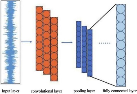
The structure of a CNN mainly consists of an input layer, convolutional layers, pooling layers, fully connected layers, and an output layer [15-16]. The convolutional layers are responsible for feature extraction from the input signal, and their operation can be expressed as shown in Eq. (1):

where $f$ denotes the activation function; $M_j$ represents the input operation; $l$ is the length of the input; $X_i^{l-1}$ refers to the target input region for convolution; $W_{ij}^l$ is the convolution kernel (also known as the weight); and $b_j$ is the bias coefficient corresponding to the convolution kernel.

The pooling layer functions to downsample the feature sequence extracted from the convolutional layer, preventing overfitting and reducing the computational complexity of the neural network [17]. Max pooling is commonly used for downsampling, and its operation can be expressed as follows:

where $y_i^l$ represents the output value of the current layer neuron; $maxpooling$ denotes the downsampling function, which selects the maximum value; $scale$ indicates the size of the pooling region; and $stride$ refers to the number of pooling strides.

The fully connected layer serves to integrate the features extracted from the convolutional and pooling layers, enabling accurate recognition of the target being detected [18-19]. It also transforms multi-dimensional inputs into a one-dimensional output, yielding the final classification result.

The output layer typically employs a Softmax classifier to produce the classification labels. The overall structural diagram of the CNN model is shown in Fig. 1.

Fig. 1Structural diagram of the CNN algorithm

When applying CNN to the fault diagnosis of automobile gearbox bearings, the inherent model architecture reveals several limitations in handling such complex mechanical signals [20]. These limitations can be summarized in the following two aspects:

On the one hand, the model architecture is static and lacks adaptive inference capability [21]. Once a traditional CNN is trained, its network structure and computation path are fixed. This “one-size-fits-all” forward propagation mechanism cannot dynamically adjust the depth or breadth of feature extraction based on variations in fault type, severity, or signal-to-noise ratio. When processing full life-cycle gearbox bearing data – from early weak faults to severe impact faults – the static model struggles to perform targeted or “triage-style” computation, leading to inefficient resource utilization and limited sensitivity to critical fault features.

On the other hand, the feature perception dimension is limited, with insufficient use of multi-domain information [22]. Conventional CNN mainly learn discriminative features from either the time or frequency domain. However, for periodic impact-type faults caused by localized damage, instantaneous phase information is equally crucial for accurate diagnosis. Existing models are often insensitive to this dimension, making it difficult to detect patterns embedded in phase relationships. Moreover, under the gearbox’s strong inherent noise and complex variable operating conditions, such single-domain representations exhibit poor robustness, thus constraining the model’s generalization ability in real industrial environments.

To overcome the above limitations, this study proposes an improved CNN model that integrates a dual-stage dynamic sparse activation mechanism with a time-frequency-phase three-dimensional attention module. The goal is to enable adaptive computation path selection based on the characteristics of each input sample, thereby enhancing the model’s computational efficiency and feature focusing capability. Meanwhile, the 3D attention module performs deep perception and fusion of the joint features constructed from the time, frequency, and instantaneous phase domains via Hilbert transform. This allows the model to fully capture and integrate multi-domain fault information, significantly improving its discriminative power and diagnostic robustness under complex operating conditions.

(1) Dual-Stage Dynamic Sparse Activation Mechanism.

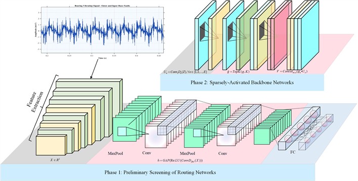
The dual-stage dynamic sparse activation mechanism is an efficient inference technique for neural networks. Its core idea is to decouple forward inference into two consecutive stages. This preserves accuracy while sharply reducing compute load and energy use. Inspired by mixture-of-experts, we design a routing–expert dynamic inference framework. The mechanism introduces conditional computation into a conventional CNN. A static network becomes a dynamic one. The routing network is a lightweight auxiliary module. It quickly estimates the health state class of the input signal and provides the route for subsequent fine diagnosis. The computational workflow of the dual-stage dynamic sparse activation is shown in Fig. 2. Below we give a detailed analysis of the computation steps for this mechanism.

Stage I employs the routing network for preliminary screening, with the detailed steps as follows:

Step 1: Input signal and processing.

The original one-dimensional vibration signal is segmented into samples of fixed length:

Step 2: Rapid Feature Extraction.

A shallow convolutional layer combined with global average pooling is used to extract compact features:

where $X\in R^L$ denotes the input one-dimensional vibration signal sample; $Conv1D_{fast}$ represents the 1D conolution layer with a very small number of filters, used to quickly capture global patterns; $GAP$ stands for global average pooling; and $h\in R^d$ denotes the extracted compact feature vector.

Step 3: Routing weight calculation:

where $W_r\in R^{E\times d}$ denotes the learnable weight matrix of the routing network; $b_r\in R^E$ represents its learnable bias vector; and $E$ is the total number of experts in the main network.

Fig. 2Computational workflow of the dual-stage dynamic sparse activation mechanism

Stage II dynamically and sparsely activates specific computation paths in selected CNN backbone layers based on the routing weights. The detailed steps are as follows:

Step 1: Expert layer construction.

The standard convolution in a specific CNN backbone layer is replaced with an expert layer. The output channels of this layer are evenly divided into $E$ groups, with each group regarded as an expert. The computation of the $e$-th expert is defined as:

where $Z\in R^{C\times T}$ denotes the input feature map of the expert layer, and $Con{v}_1{D}_e$ represents the output feature map produced by the $e$-th expert.

The determination of the total number of experts $E$ mainly depends on the complexity of fault characteristics and the capacity requirement of the model. If the task involves complex patterns such as multiple fault types and multiple damage levels, a larger value of $E$ is required to provide sufficient feature representation capability. At the same time, the value of $E$ should also take into account the number of model parameters and the available computational resources. In practice, $E$ can usually be designed as a grouping factor of the feature-channel number, and its optimal value can be selected within a typical range through ablation experiments.

Step 2: Expert activation.

To achieve high computational efficiency and mimic a triage-like decision process, only the top $K$ experts with the highest routing weights are activated for inference:

where, $TopK(,K)$ denotes the operator that retains only the top $K$ values in the input vector while setting the rest to zero, and $\tilde{g}$ represents the sparsified gating vector.

The selection of the number of activated experts $K$ is directly related to inference efficiency and dynamic adaptability. To achieve significant computational compression, $K$ should be much smaller than $E$, so that more than 80 % of the computational cost can be saved. The specific value of $K$ should be determined according to the discriminative strength of the fault features. When the feature categories are clearly separable, a smaller $K$ can be chosen so that the model focuses on the most discriminative experts. When the features are strongly coupled, $K$ may be appropriately increased to fuse multi-path information. In addition, $K$ can be further fine-tuned dynamically according to the entropy of the routing-network output weights, thereby enhancing the adaptability of the expert-selection process.

Step 3: Weighted aggregation and output.

The outputs of all activated experts are weighted by their corresponding routing coefficients and concatenated along the channel dimension to form the final output of the expert layer:

where $Concat$ denotes the concatenation operation along the channel dimension.

(2) Time-Frequency-Phase 3D Attention Module.

Conventional attention mechanisms are typically confined to either the time or frequency domain, overlooking the periodic fault impulses that recur along the phase axis of an automotive gearbox – a pattern that is crucial for locating subtle faults under heavy noise conditions.

First, for each channel $f_c$ in the 2D feature map extracted by the CNN, the analytic signal is constructed using the Hilbert transform to incorporate instantaneous phase information:

where $H\left\{\right\}$ denotes the Hilbert transform, $f_c^a\left(t\right)$ represents the analytic signal in complex form, and $j$ is the imaginary unit.

Next, the instantaneous amplitude and instantaneous phase are extracted from the analytic signal to construct a three-dimensional feature tensor:

where $Norm\left(F\right)$ denotes the normalized original feature map; $A$ represents the instantaneous amplitude matrix formed by stacking all channels; $\cos ({\mathrm{\Phi }}_c)$ is the stacked matrix; $Stack\left(\right)$ denotes the stacking operation along the new dimension; and $T$ is the constructed three-dimensional feature tensor, where the three dimensions correspond to channel, time, and phase.

The mapping relationship among the channel dimension, time dimension, and phase dimension reflects a three-dimensional collaborative representation mechanism. The channel dimension provides multiple feature perspectives, the time dimension records the dynamic evolution process, and the phase dimension supplements the fine description of oscillatory structures. In the three-dimensional attention module, this mapping relationship is realized by computing attention weights along parallel branches for each dimension, thereby achieving cross-dimensional feature recalibration. Specifically, by computing correlations in the joint channel-time-phase space, the model is able to focus on those feature regions that exhibit strong fault sensitivity at specific channels, time points, and phase positions. In this way, deep fusion and enhanced perception of multi-domain fault information are achieved.

The channel description vector and the corresponding channel-attention weights are calculated as follows:

where $W_{c1}$ and $W_{c2}$ are the weight matrices of two fully connected layers; $r$ denotes the reduction ratio; $\delta$ represents the ReLU activation function; and $a_c\in R^C$ is the computed channel attention weight vector.

The computation formula for the temporal attention branch is defined as follows:

where $z_t\in R^T$ denotes the temporal descriptor vector obtained through global average pooling along the channel and phase dimensions; $W_{t1}$, $W_{t2}$ represents the weight matrix; and $a_t\in R^T$ is the resulting temporal attention weight vector.

The computation formula for the phase attention branch is defined as follows:

where $z_p\in R^3$ denotes the phase descriptor vector obtained through global average pooling along the channel and time dimensions; $W_p\in R^{3\times 3}$ represents the weight matrix of the fully connected layer; and $a_p\in R^3$ is the resulting phase attention weight vector.

Finally, the attention weights from the three dimensions are broadcast to match the size of the original feature tensor and multiplied element-wise to achieve feature recalibration:

where $\otimes$ denotes the element-wise multiplication with broadcasting, and $\tilde{T}$ represents the enhanced feature tensor weighted by the 3D attention mechanism.

The final output of this module is the refined two-dimensional feature map $\tilde{F}$.

2.2. Transformer model

The Transformer model is a deep learning architecture based on the self-attention mechanism. Its core idea is to capture global dependencies among elements within a sequence through self-attention [23-24]. To adapt the data to the Transformer’s sequence processing capability, the feature maps must first be converted into sequential form, as shown in Eq. (20):

where $P$ denotes the time length of each block; $N$ represents the total number of blocks; and $P_i$ indicates the $i$-th feature block.

Then, each feature block is flattened into a vector and projected into the hidden dimension $D$ through a linear transformation:

where $Flatten\left(\right)$ denotes the operation that flattens the matrix into a vector; $p_i\in R^{CP}$; $W_p$ represents the projection weight matrix; $b_p$ is the projection bias vector; and $e_i\in R^D$ refers to the embedding vector of the $i$-th block.

Since the Transformer model itself lacks positional awareness, positional encoding is introduced to explicitly inject sequence order information, as shown in Eq. (23):

where $E_p\in R^{(N+1)\times D}$ denotes the positional encoding matrix, and $p_j\in R^D$ represents the positional encoding vector of the $j$-th position, which is a learnable parameter.

The block embeddings are added to the positional encodings to form the input sequence of the Transformer model:

where $S_0$ represents the input sequence matrix of the Transformer, and $[;]$denotes the concatenation operation along the sequence dimension.

The Transformer encoder is composed of $L$ identical layers, each containing two core sub-layers [25]. The multi-head attention mechanism of the Transformer encoder is illustrated in Fig. 3.

The first sub-layer is the multi-head self-attention mechanism, which applies linear transformations to the input sequence $S_{l-1}$ to generate the query, key, and value matrices:

where $W^Q$, $W^K$, and $W^V$ represent the weight matrices for the query, key, and value, respectively; $d_k$ denotes the dimension of each attention head; and $H$ is the total number of attention heads.

Fig. 3Flowchart of the multi-head attention mechanism

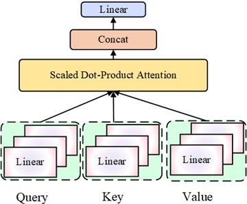
The computation formula for the scaled dot-product attention is defined as follows:

where $Q{K}^T$ represents the computation of correlation scores between all sequence position pairs; $\sqrt{d_k}$ is the scaling factor used to prevent excessively large dot products that could cause gradient vanishing; and $soft\mathit{max}()$ denotes the process of converting correlation scores into attention weights, where each position in the output matrix is a weighted sum of the value vectors, with weights determined by their corresponding attention scores.

The concatenation and projection computation of the multi-head attention mechanism is defined as follows:

where $MSA\left(S_{l-1}\right)$ denotes the final output of the multi-head attention mechanism; $hea{d}_h$ represents the output of the $h$-th attention head; and $W^O$ is the output projection matrix.

The computation formulas for residual connection and layer normalization are defined as follows:

where $LayerNorm\left(\right)$ denotes the layer normalization operation, which normalizes the vector of each sequence; and $Z_l$ represents the output of the first sub-layer.

The second sub-layer is a feed-forward neural network (FFN), whose two-layer MLP transformation is computed as follows:

where $W_1$ and $W_2$ represent the weights and biases of the first and second layers, respectively.

The computation formulas for the second residual connection and layer normalization are expressed as follows:

where $S_l$ denotes the final output of the $l$-th layer of the Transformer encoder.

After processing through $L$ layers of Transformer encoders, the model maps the input sequence into multi-level semantic representations. From the final layer output, the vector corresponding to the [CLS] token is extracted as the global semantic representation of the entire input sequence [26]. Specifically, $S_{\left[CLS\right]}^L\in R^D$ denotes the final representation of the [CLS] token, which contains the compressed information of the whole sequence.

The computation formula for the classification layer is defined as follows:

where $W_{cls}$ denotes the weight matrix of the classification layer; $b_{cls}$ represents the bias vector; $M$ is the total number of fault categories; and $y_{pred}$ is the predicted fault probability distribution of the model.

2.3. A hybrid improved CNN-Transformer architecture for automotive gearbox bearing fault diagnosis

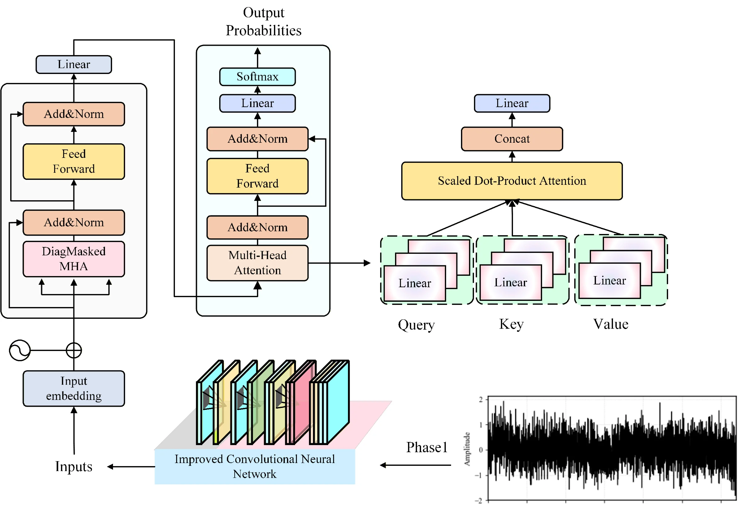
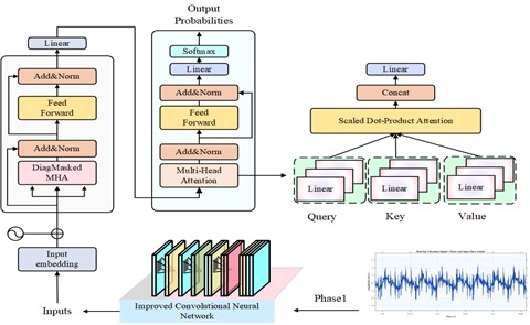
The improved CNN-Transformer hybrid diagnostic model proposed in this study adopts an end-to-end hierarchical architecture, which is composed sequentially of an input preprocessing module, a two-stage dynamically sparse-activated CNN module, a time-frequency-phase three-dimensional attention module, a serialization and positional-encoding module, a Transformer encoder module, and a classification output module. First, the input preprocessing module standardizes and formats the raw vibration signals to construct sample batches with a unified size. Then, the two-stage dynamically sparse-activated CNN module uses a routing network to rapidly evaluate the input features and dynamically activate only part of the expert layers in the backbone network, thereby realizing adaptive feature extraction. Next, the time-frequency-phase three-dimensional attention module applies a Hilbert transform to the extracted two-dimensional feature maps to construct a three-dimensional tensor along the channel, time, and phase dimensions, and fuses and refines multi-domain features through parallel attention branches. After that, the serialization and positional-encoding module divides the refined features into sequential blocks and adds learnable positional encodings, converting them into an input sequence suitable for the Transformer. The Transformer encoder module captures global dependencies within the sequence through multiple layers of self-attention and feed-forward networks, thereby extracting global semantic representations. Finally, the classification output module maps the global representation to the probability distribution of fault categories to complete the diagnostic decision. The entire model is trained in an end-to-end manner using the cross-entropy loss function. The AdamW optimizer together with a cosine-annealing learning-rate scheduler is adopted to optimize the network, while Dropout and weight decay are employed to enhance generalization performance. In this way, the proposed method achieves high diagnostic accuracy and strong robustness for transmission-bearing fault diagnosis while maintaining computational efficiency.

The 2D feature map is fed into the Transformer model, where sequential embedding connects the dynamic activation and multi-dimensional attention modules. The model first performs efficient triage-style inference, then enhances its sensitivity to fault-related features of automotive gearbox bearings. This design ensures a balance between computational efficiency and feature discriminability, improving diagnostic performance under complex operating conditions. The computational steps of the improved CNN-Transformer-based gearbox bearing fault diagnosis model are as follows:

Step 1: Input signal preprocessing and batch construction.

Collect the raw one-dimensional vibration acceleration signals of automotive gearbox bearings under different health conditions, such as normal, inner race fault, outer race fault, and rolling element fault. The continuous signal is segmented into fixed-length samples, each associated with a fault label. All samples are then normalized to have a mean of 0 and a standard deviation of 1 to accelerate model convergence.

Step 2: Adaptive feature extraction and refinement.

Feed the data into the routing network to obtain compact feature vectors. Pass these vectors through a fully connected layer to compute the initial routing weights, followed by sparse gating operations. Simultaneously, input the data into the CNN backbone to generate a 2D feature map. Using the time-frequency-phase 3D attention module, construct analytic signals for each channel of the 2D feature map. Extract the instantaneous amplitude and phase from these analytic signals, compute the 3D attention weights, and broadcast them to match the shape of the 3D feature tensor. Then, perform element-wise multiplication and average the weighted 3D tensor along the “source” dimension to reduce it back to a 2D feature map, completing the feature refinement process.

Step 3: Sequence modeling and classification.

The refined 2D feature map is serialized into block embedding vectors. Positional encodings and class information are then added to these embeddings to form the Transformer’s input sequence. The sequence is fed into the Transformer, and finally, the Softmax function outputs the predicted probability distribution for each fault category.

The computational workflow of the improved CNN-Transformer-based gearbox bearing fault diagnosis model is illustrated in Fig. 4.

Fig. 4Improved CNN-Transformer-Based fault diagnosis model for automotive gearbox bearings

3.1. Data sources

The experimental data used in this study come from a vibration signal dataset of automotive gearbox rolling bearings independently constructed by the research team. The dataset was collected using the comprehensive gearbox bearing fault test bench shown in Fig. 5, which enables precise simulation of the actual operating conditions of gearbox bearings.

Fig. 5Comprehensive experimental test bench for automotive gearbox bearing faults

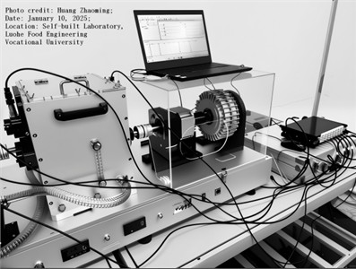
The experiment used NU206 cylindrical roller bearings, commonly found in automotive gearboxes, as the test objects. Using laser engraving technology, four typical fault modes were introduced at critical bearing components: rolling element fault, inner race fault, outer race fault, and cage fault. For the first three localized fault types, the damage diameters were set to 0.2 mm, 0.4 mm, and 0.6 mm, representing the progression from early minor damage to severe failure. The cage fault was categorized into three levels – slight, moderate, and severe – based on the degree of material wear. Additionally, the dataset includes vibration signals from healthy bearings without defects, serving as baseline samples for fault diagnosis.

During data collection, the experimental setup was configured to simulate real gearbox operating conditions. The spindle speed of the test bench was set to 1000 rpm, 1400 rpm, 1800 rpm, and 2200 rpm, representing different vehicle driving speeds. The load was applied using a magnetic powder brake, with torque levels of 1.5 N·m, 3.0 N·m, and 4.5 N·m, corresponding to varying gearbox load conditions. Vibration signals were captured using dual-axis ICP acceleration sensors mounted on both the radial and axial sides of the gearbox bearing seat, allowing simultaneous acquisition of two-directional vibration responses to enhance fault information completeness. Data acquisition was performed using a NI-9234 dynamic signal acquisition module, with a sampling frequency of 64 kHz, ensuring full capture of high-frequency impact components and harmonic features generated by bearing faults. Each experiment recorded 15 seconds of continuous data, during which all operating parameters were kept stable. The detailed structure of the dataset is presented in Table 1.

The proposed model can be directly applied to bearings with different fault types within the defect-size range of 0.2-0.6 mm. Moreover, variations in sensor placement, sampling frequency, and fault-induction methods have almost no impact on the performance of the model, and high diagnostic accuracy can still be maintained. When applying the model to other datasets, only minor adjustments to the data format and the correspondence between the input and output interfaces are required.

3.2. Experimental environment

To verify the effectiveness of the proposed improved CNN-Transformer-based fault diagnosis model for automotive gearbox bearings, this section provides a detailed description of the experimental hardware and software environment, key hyperparameter settings, and training configurations. The dataset was divided into training, validation, and test sets with a ratio of 6:2:2. All experiments were conducted under the same unified environment to ensure the reproducibility and fairness of the results.

The host system was equipped with an NVIDIA GeForce RTX 5090 GPU, which offers exceptional parallel computing performance. Its powerful computational capability accelerates complex operations such as matrix multiplication and convolution, significantly reducing model training time and enabling a large number of experimental iterations within a relatively short period. When processing large-scale vibration signal data from automotive gearbox bearings, the RTX 5090 GPU provides efficient data processing and analysis support, ensuring high-performance model training.

The operating system used was Ubuntu 20.04 LTS, chosen for its open-source nature, stability, and excellent compatibility with various development tools and libraries.

Given the characteristics of the constructed automotive gearbox bearing vibration dataset – including multiple fault types, varying damage severities, and complex operating condition combinations – the Transformer model’s key hyperparameters were carefully tuned to balance feature extraction capability and computational efficiency, while accounting for the non-stationary nature of vibration signals and the time-frequency structure of fault features. The core hyperparameter settings are described as follows:

First, in terms of input representation, to adapt to the high sampling frequency (64 kHz) and sample length (4096 points) of the vibration signals, the input sequence length was set to 4096. An overlapping segmentation strategy was applied to divide the raw signal into fixed-length subsequences, enhancing the continuity of temporal features. Meanwhile, since the dataset includes dual-channel vibration signals from both radial and axial directions, the model input dimension was set to 2, allowing full use of the complementary information provided by multiple sensors.

Next, in the design of the Transformer encoder, the number of attention heads was set to 8 to capture fault-sensitive features across different frequency bands and time scales. This configuration takes into account the sparsity of fault impulses in the time domain and the local correlation of high-frequency resonance features. The hidden dimension was set to 512, providing sufficient feature representation capacity to model the nonlinear evolution of gearbox bearing faults from early weak defects to severe failures. The encoder depth was optimized to 6 layers, allowing the network to extract deep hierarchical features while avoiding training instability and overfitting risks associated with overly deep models.

Then, in the feed-forward neural network (FFN) module, an intermediate layer with a dimension of 2048 was used to enhance the model’s ability to fit the modulated components and harmonic structures in vibration signals through nonlinear transformations. Both the attention dropout and feed-forward dropout rates were set to 0.1, improving the model’s generalization performance under complex conditions such as variable speed and load. The AdamW optimizer was adopted with an initial learning rate of 1e-4, combined with a cosine annealing learning rate schedule to ensure smooth convergence and avoid local minima.

Finally, the model’s output layer corresponds to 13 fine-grained health states, covering five fault categories, including the normal condition and multiple damage levels. A Softmax function is applied to achieve end-to-end fault classification. This combination of hyperparameters was validated through ablation experiments, demonstrating its ability to effectively extract discriminative fault features from high-dimensional vibration signals and provide a robust feature representation foundation for deep transfer learning tasks.

3.3. Time-frequency analysis of vibration signals from automotive gearbox bearings

To visually demonstrate the vibration characteristics of automotive gearbox bearings under different conditions and to verify the effectiveness of the improved CNN in fault feature extraction, this section performs time–frequency analysis on the raw vibration signals. Time-frequency analysis reveals the energy distribution of signals across both the time and frequency domains, serving as a crucial tool for identifying fault-induced impact components and their corresponding resonance frequencies in non-stationary signals.

Fig. 6Time-frequency analysis results of the self-built automotive gearbox bearing dataset

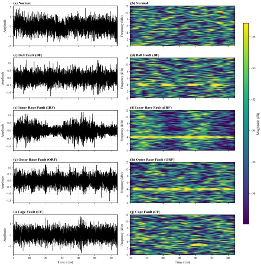
Representative vibration signals were selected under identical operating conditions (1800 rpm, 2 hp) for four bearing states: Normal, Ball Fault (0.3556 mm), Inner Race Fault (0.3556 mm), and Outer Race Fault (0.3556 mm). The analysis results are shown in Fig. 6.

As shown in Fig. 6, the time-domain waveform of the normal state (a) exhibits stable random oscillations with small amplitude fluctuations and no obvious impulsive changes, reflecting a steady dynamic response under healthy conditions. In contrast, the waveforms of the ball fault (c), inner race fault (e), outer race fault (g), and cage fault (i) show significant impulsiveness and non-stationarity, characterized by numerous pulse-like amplitude spikes. This occurs because faults in components such as the rolling elements, inner race, outer race, and cage cause periodic impacts as they rotate, resulting in intermittent bursts of vibration energy in the time domain – directly indicating how these faults disturb the vibration pattern of the bearing.

From the frequency-domain analysis, the normal state (b) shows a smooth and evenly distributed energy spectrum, dominated by broadband components with no distinct energy peaks – demonstrating the typical “broadband steady vibration” characteristics of a healthy bearing. In contrast, under fault conditions (d, f, h, j), the time-frequency plots display pronounced energy peaks at specific frequencies corresponding to the characteristic fault frequencies and their harmonics. For example, in the time-frequency maps of the ball fault, inner race fault, outer race fault, and cage fault, the energy concentration around these characteristic frequencies becomes clearly visible. This phenomenon results from the periodic impact excitations caused by faults, which generate harmonic components within the system. Consequently, the time-frequency energy distribution becomes dominated by fault characteristic frequencies, confirming the effectiveness of time-frequency analysis in identifying the frequency components associated with different bearing fault types.

3.4. Ablation experiment

To verify the effectiveness and necessity of each improved module proposed in this study – namely, the dual-stage dynamic sparse activation mechanism and the time-frequency-phase 3D attention module – a systematic ablation experiment was conducted. The experiments were performed on the self-built automotive gearbox bearing dataset described in Section 3.1. All comparative models were trained under identical experimental environments and hyperparameter configurations (Section 3.2) to ensure fair comparison. Four model variants were designed for evaluation:

Model 1: CNN. CNN serves as the baseline model, using only a conventional convolutional neural network for feature extraction. It does not include the dynamic sparse activation mechanism or the multi-dimensional attention module.

Model 2: CNN + DSAM. Based on the CNN architecture, the Dual-Stage Dynamic Sparse Activation Mechanism (DSAM) is introduced to verify its effectiveness in enabling adaptive computation and improving computational efficiency.

Model 3: CNN + DSAM + TFP-Attention. Building upon Model 2, this variant further introduces the Time-Frequency-Phase 3D Attention (TFP-Attention) module to verify its contribution to multi-domain feature perception and feature refinement.

Model 4: Improved CNN–Transformer. This is the complete model proposed in this study. It integrates Model 3 with the Transformer encoder to verify the improvement in final diagnostic performance achieved through global dependency modeling. The results of the ablation experiment are shown in Fig. 7.

In terms of the loss curves, both the training loss (Fig. 7(a)) and validation loss (Fig. 7(b)) of all models converge as the number of epochs increases. The Improved CNN-Transformer shows the lowest loss, followed by CNN + DSAM + TFP-Attention, CNN + DSAM, and the baseline CNN with the highest. For the accuracy curves, both training accuracy (Fig. 7(c)) and validation accuracy (Fig. 7(d)) rise steadily with epochs, where the Improved CNN-Transformer consistently achieves the highest accuracy. These results indicate a step-wise improvement as the DSAM and TFP-Attention modules are introduced and further integrated with the Transformer architecture. The enhanced model demonstrates clear advantages in minimizing loss, improving classification accuracy, and strengthening generalization performance, confirming the effectiveness of each proposed module.

Fig. 7Results of the ablation experiment

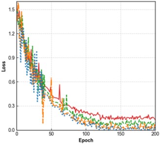
a) Training loss

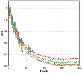
b) Validation loss

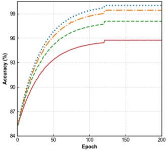
c) Training accuracy

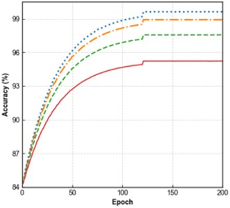
d) Validation accuracy

Table 2 summarizes the fault diagnosis performance of different model variants on the test set. The evaluation metrics include overall accuracy, precision, recall, F1-score and average inference time.

Table 2 clearly illustrates the evolutionary path from the baseline CNN to the proposed Improved CNN-Transformer model. The overall accuracy increases from 94.16 % to 99.73 %, while all other metrics exceed 99.6 %. This demonstrates the model’s exceptional ability to capture and distinguish complex gearbox bearing fault features. Its high precision minimizes unnecessary maintenance, high recall prevents missed fault detections, and the balanced F1-score confirms robust overall performance. Collectively, these results show that the proposed approach offers a reliable technical solution to the core industrial challenge of achieving zero false alarms and zero missed detections in intelligent fault diagnosis.

3.5. Comparative experiments of different fault diagnosis algorithms

To comprehensively evaluate the overall performance of the proposed method, this section conducts comparative experiments with several state-of-the-art fault diagnosis algorithms. All methods are tested on the self-built automobile gearbox bearing dataset, using the same data partitioning scheme to ensure fairness and consistency. The compared algorithms include GDS-YOLOv5s, MCWT-WCFormer, NA-MVMD-ALCAT, and the proposed method. The experimental results are presented in Fig. 8.

Fig. 8Experimental comparison of evaluation metrics across different fault diagnosis algorithms

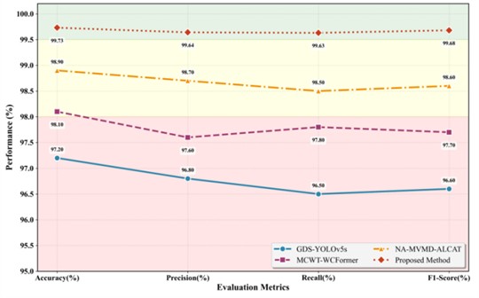
As shown in Fig. 8, the proposed method achieves the best performance across all four key evaluation metrics – accuracy, precision, recall, and F1-score – demonstrating superior and well-balanced diagnostic capability. Specifically:

(1) In terms of overall accuracy, the proposed method achieves 99.73 %, outperforming the best competing model (NA-MVMD-ALCAT) by 0.83 %. More importantly, it maintains the highest classification accuracy across all five operating conditions, significantly surpassing the other advanced diagnostic models. This result demonstrates the method’s exceptional adaptability to varying working environments and its strong generalization capability under complex operational conditions.

(2) In terms of fault discrimination precision, the proposed method achieves a precision of 99.64 %, significantly higher than all comparison algorithms. This indicates that the model rarely misclassifies normal or other fault states as specific failures during diagnosis, thereby effectively controlling the risk of false positives. Such precision is of great engineering importance, as it helps prevent unnecessary maintenance downtime and ensures operational continuity.

(3) In terms of fault recognition completeness, the proposed method achieves a recall of 99.63 %, outperforming models such as NA-MVMD-ALCAT. This demonstrates the model’s stronger ability to capture true fault samples, significantly reducing the probability of missed detections (false negatives). Such performance is critical for enabling early fault warning and preventing catastrophic failures in real-world industrial systems.

(4) In terms of overall performance, the proposed method achieves an F1-score of 99.68 %, representing a well-balanced harmonic mean of precision and recall. This result further confirms that the model attains an optimal trade-off and synergy among multiple evaluation metrics, ensuring robust and reliable classification performance across varying fault conditions.

In summary, the experimental results consistently demonstrate that the proposed hybrid diagnostic model excels in the fault diagnosis of automotive gearbox bearings. It not only achieves superior overall performance but also significantly reduces both false alarms and missed detections, highlighting its robustness and reliability. These findings confirm the model’s effectiveness and competitiveness, providing a solid foundation for its practical deployment in complex industrial environments.

Fig. 9Confusion matrices of gearbox fault diagnosis results for different algorithms

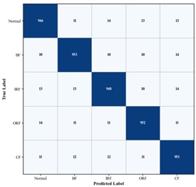
a) CNN. Accuracy 94.16 %

b) CNN+DSAM. Accuracy 96.23 %

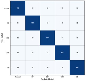
c) CNN+DSAM+TEP-Attention. Accuracy 98.76 %

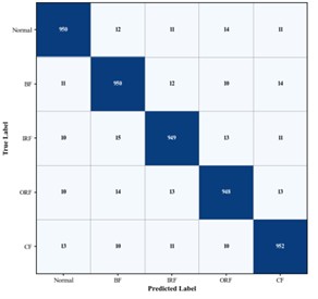
d) Improved CNN-Transformer. Accuracy 99.73 %

As shown in Fig. 9, the diagonal elements of the confusion matrix represent the number of samples correctly classified for each condition, while the off-diagonal elements indicate misclassified samples. In the confusion matrix of the proposed method, nearly all predictions for the five operating conditions are concentrated along the diagonal, indicating exceptionally high classification accuracy. This demonstrates that the model can precisely capture the distinguishing features of various gearbox states – including normal operation and the three typical fault types. In summary, the proposed method demonstrates superior performance across all gearbox bearing fault diagnosis experiments, consistently outperforming current state-of-the-art diagnostic approaches.

3.6. Hyperparameter analysis

To investigate the influence of the total number of experts E and the number of activated experts $K$ on the diagnostic performance of the proposed model, a series of hyperparameter analysis experiments were conducted. All experiments were carried out on the self-constructed dataset used in this study. The experimental results are shown in the following figures.

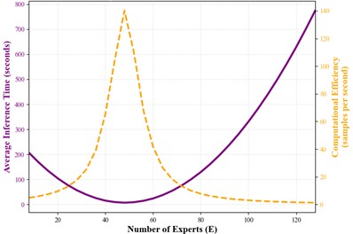
The upper part of the figure illustrates that the ratio K/E is a key regulator for balancing model accuracy and computational cost. The horizontal axis represents the K/E ratio, while the vertical axis denotes model accuracy. Three representative curves are presented, corresponding to model configurations with “high discriminability-low coupling”, “moderate discriminability-moderate coupling,” and “low discriminability-high coupling”. The overall trend shows that, as K/E increases (that is, more experts are activated), the model accuracy generally improves, with the high-discriminability and low-coupling configuration achieving the best performance. Two key regions are highlighted in the figure. When K/E is small, the system lies in the “inference-time priority” region, where the computational speed is high but the accuracy is limited. As K/E increases to a moderate range, the system moves into the “computational-efficiency optimum” region, where relatively high accuracy can be achieved while keeping the computational cost under control.

Fig. 10Results of the parameter analysis experiments

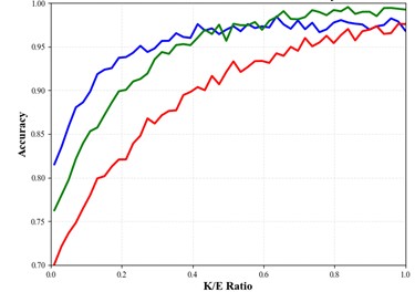
a) Effect of K/E ratio on model accuracy

b) Effect of expert number on inference performance

The lower part of the figure further analyzes the influence of the total number of experts (E) on the actual inference performance. The horizontal axis denotes the number of experts, while the vertical axis represents the average inference time. The expected trend is that inference time does not improve linearly with the increase of E. When the number of experts is small, increasing E may enhance the model capacity and processing ability, potentially resulting in speed gains or only a mild increase in latency. However, once the number of experts exceeds a certain threshold, the complexity of routing decisions, memory-access latency, and communication overhead increase significantly, which leads to a rapid rise in the average inference time. This indicates that blindly increasing the number of experts is not desirable and must be considered jointly with the activation ratio K/E.

In summary, the figure provides clear guidance for the design of mixture-of-experts models: model performance must be carefully balanced among accuracy, speed, and computational efficiency. For resource-constrained scenarios, it is preferable to adopt a relatively small total number of experts (E) combined with a moderate activation ratio (K/E). For cloud-based scenarios where maximum accuracy is required, a larger E and a higher K/E ratio may be selected, but the corresponding latency and computational cost must be accommodated.