Rolling bearing fault diagnosis under varying operating conditions using a convolutional-Transformer multi-alignment approach

Wang, Yiying; Sui, Fulu; Li, Xiaoling; Zhang, Xiaoxin; Liu, Mingxian; Liu, Chen; Wu, Jie

doi:10.21595/jve.2025.25460

Journal of Vibroengineering

Browse Journal

Submit article

Published: February 21, 2026

Check for updates

Rolling bearing fault diagnosis under varying operating conditions using a convolutional-Transformer multi-alignment approach

Yiying Wang¹

Fulu Sui²

Xiaoling Li³

Xiaoxin Zhang⁴

Mingxian Liu⁵

Chen Liu⁶

Jie Wu⁷

^{1, 2, 3, 4, 5, 6, 7}Handan Vocational College of Technology, Handan, China

Corresponding Author:

Xiaoxin Zhang

Cite the article Download PDF

Article in Press

Downloads 38

Abstract

In this study, a novel deep transfer learning method, termed the Universal Domain Alignment and Multi-level Alignment Network (UDAM-Net), is established to address the significant feature distribution discrepancy between the source and target domains caused by the difficulty of feature extraction for rolling bearings under complex operating conditions. In the feature extraction stage, a one-dimensional convolutional neural network is integrated with a Transformer-based multi-head attention mechanism to effectively enhance the feature representation capability of raw signals. Additionally, the complementary advantages of Joint Maximum Mean Discrepancy (JMMD), Multi-kernel Maximum Mean Discrepancy (MK-MMD), and a domain discriminator are explored by designing a collaborative mechanism combining distribution metrics and adversarial learning in conjunction with transfer learning. Furthermore, an uncertainty-based weighting strategy is introduced to adaptively adjust the loss function and dynamically balance the contributions of different alignment modules. Finally, the Adam optimizer is employed to accelerate model convergence. Experimental results on the CWRU public dataset and a laboratory-built test rig dataset demonstrate that UDAM-Net achieves classification accuracies of 96.67 % and 96.17 %, respectively. This study enlightens fault diagnosis based on feature extraction and cross-domain feature alignment.

Rolling bearing fault diagnosis under varying operating conditions using a convolutional-Transformer multi-alignment approach

Highlights

A multi-scale feature extraction framework is built by integrating a Transformer with a one-dimensional CNN. Local temporal features and global dependencies are jointly modeled, improving long-range feature learning and robustness under varying operating conditions.
JMMD, MK-MMD, and a domain discriminator are jointly integrated to achieve multi-dimensional alignment of marginal distributions, conditional distributions, and discriminative features, contributing to mitigated distribution shift between domains and enhanced model generalization capability.
An uncertainty-adaptive loss weighting strategy dynamically balances multiple loss terms, avoiding manual hyperparameter tuning. Combined with the Adam optimizer, it improves training stability, convergence speed, and model robustness under noisy and cross-operating conditions.

1. Introduction

While rolling bearings are critical components in rotating machinery, their wide range of use and harsh operating conditions make them one of the most failure-prone components in such practical industrial systems. Since mechanical equipment typically operates under varying working conditions, conducting rolling bearing fault diagnosis under complex operating conditions is of great significance for engineering applications [1, 2].

In traditional learning-based approaches, literature [3] utilized nonlinear dimensionality reduction methods, including Diffusion Maps, Locally Linear Embedding (LLE), and Autoencoders, to lessen signal dimensionality and extract features, followed by fault identification through GK clustering and k-medoids. literature [4] proposed a CEEMDAN-IWSO-VMD-based denoising method, in which secondary signal decomposition was performed with CEEMDAN and VMD, and statistical features were subsequently extracted and fed into a BiLSTM network for fault identification. However, the above-mentioned methods rely heavily on signal decomposition for denoising and fault feature enhancement under practical operating conditions, hindering the direct extraction of discriminative features from raw vibration signals. Moreover, these methods strongly depend on manual parameter tuning, degrading feature quality and leading to issues such as mode mixing, over-decomposition, and high computational complexity. This limits their applicability to complex signals under varying operating conditions.

To overcome the aforementioned limitations, literature [5] leveraged the advantages of convolutional neural networks (CNN) in spatial feature extraction, noise robustness, and computational efficiency to improve the accuracy of bearing fault diagnosis. literature [6] proposed a hybrid method combining CNNs with long short-term memory (LSTM) networks to capture temporal dependencies in the data, followed by fault diagnosis through an optimized least squares support vector machine. While CNNs can automatically extract local features and reduce the reliance on manual feature engineering, their receptive fields are constrained by kernel size and network depth, rendering it difficult to capture long-range global temporal dependencies. Existing studies have combined CNNs with LSTM or GRU networks, whereas such architectures generally suffer from low training efficiency when handling long sequences and features under complex operating conditions. In contrast, the self-attention mechanism of the Transformer allows for the computation of dependency weights between arbitrary positions, enabling the integration of global temporal features.

For example, literature [7] first mapped time-domain vibration signals into the frequency domain using the fast Fourier transform (FFT) and employed CNNs to process time-frequency representations and extract local impulsive patterns and frequency energy distributions. Moreover, they captured long-term dependencies following the Transformer’s multi-head attention mechanism, thereby improving diagnostic accuracy. With respect to feature extraction, literature [8] constructed a multi-branch Transformer network to extract global features from different perspectives and achieved fault diagnosis under noisy environments through a multi-supervision strategy combined with local feature enhancement. literature [9] decomposed raw signals through variational mode decomposition (VMD) to remove noise, extracted multi-scale features via CNNs, and employed a Transformer to capture long-range dependencies for fault diagnosis. In practical machinery operation, nevertheless, CNN-Transformer-based methods primarily focus on the fusion of local and global feature representations, and their feature alignment capability remains limited. Consequently, it is difficult to capture feature discrepancies across different samples, resulting in poor feature alignment under varying operating conditions.

Transfer learning, which is an effective approach for addressing varying operating conditions, aims to transfer knowledge from the source domain to the target domain for reducing the discrepancy between them [10]. The literature [11] employed an improved convolutional neural network to extract multi-scale features and utilized multi-kernel maximum mean discrepancy (MK-MMD) to reduce feature discrepancies between the source and target domains, contributing to the improved accuracy of cross-domain feature discrimination, literature [12] combined CNNs with an attention mechanism to enhance signal feature representation and addressed domain shift through JMMD, literature [13] applied EMD for denoising and achieved feature alignment by integrating CNNs and attention mechanisms with a domain discriminator. Although MK-MMD, JMMD, and domain discriminators can extract domain-invariant features and enhance model robustness, each of them faces inherent challenges. Specifically, JMMD suffers from high computational complexity and slow training speed, and is sensitive to multi-scale feature representations and kernel selection; MK-MMD improves flexibility but only aligns marginal distributions while neglecting conditional distributions; domain discriminators are prone to training instability or gradient vanishing, bringing about the weakened discriminative capability of learned features.

In this study, the self-attention mechanism of the Transformer is introduced to address the performance degradation of conventional CNN-based methods under varying operating conditions triggered by limited receptive fields and insufficient long-range dependency modeling. By employing a single-layer architecture, a global receptive field is achieved while noisy features are dynamically suppressed, enabling the enhancement of feature extraction capability and more robust deep representations of raw signals. With the purpose of mitigating the large feature discrepancies between the source and target domains, a joint alignment strategy integrating JMMD and MK-MMD is proposed, together with a domain discriminator for domain feature alignment. This approach overcomes the limitations of conventional metrics in computational efficiency, conditional distribution alignment, and training stability. Furthermore, the label classification loss, domain alignment loss, JMMD loss, and MK-MMD loss are dynamically balanced following an uncertainty-adaptive weighting mechanism to alleviate the issue of inconsistent loss scales and lower reliance on manual hyperparameter tuning. Furthermore, the Adam optimizer is adopted to alleviate the limitations of traditional optimization methods concerning gradient noise, sparsity, and learning rate adjustment, thereby improving training stability and convergence speed. Based on these improvements, a novel deep transfer learning framework, termed the UDAM-Net, is constructed in this study, providing a new solution for cross-domain fault diagnosis of rolling bearings.

The main contributions of this study are summarized as follows:

(1) A multi-scale joint feature extraction framework is constructed by incorporating a Transformer layer on top of a one-dimensional convolutional neural network. By integrating local temporal features with global dependency modeling, the proposed network improves long-range feature capture and alleviates insufficient feature representation under varying operating conditions.

(2) JMMD, MK-MMD, and a domain discriminator are jointly integrated to achieve multi-dimensional alignment of marginal distributions, conditional distributions, and discriminative features, contributing to mitigated distribution shift between domains and enhanced model generalization capability.

(3) An uncertainty-adaptive loss weighting strategy is employed to dynamically allocate weights among different loss components, avoiding imbalance stemming from manual hyperparameter tuning. In conjunction with the Adam optimizer, training stability and convergence speed are further improved, allowing the model to maintain robustness under noisy and cross-operating conditions.

2. Fault diagnosis model

In this study, a transfer learning-based rolling bearing fault diagnosis model is designed for varying operating conditions. First, a Transformer module is introduced on top of a 1D-CNN to reduce the excessive time consumption and manual parameter tuning arising from reliance on handcrafted feature extraction, enabling direct feature learning from raw vibration signals. Meanwhile, transfer learning is incorporated by combining explicit distance-based metrics with implicit adversarial alignment mechanisms. In this way, a cross-domain feature alignment framework is constructed, achieving class discriminability, multi-scale global feature alignment, and dynamic adaptability. Finally, an uncertainty-adaptive weighting strategy is applied to the label classification loss, JMMD loss, MK-MMD loss, and domain discriminator loss, and the Adam optimizer is employed to enhance training stability and convergence speed. The overall architecture of the proposed model is illustrated in Fig. 1. The corresponding pseudocode is detailed in Table 1.

2.1. Fault recognition classifier

This study adopts a feature extractor that combines a 1D-CNN with a Transformer. The 1D-CNN is effective at capturing local patterns in time-series signals and highlights features such as edges, peaks, and harmonic components of fault signals. Nevertheless, its receptive field is inherently limited. The Transformer can model long-range dependencies and attend to periodic patterns and strongly correlated regions from a global perspective. Unfortunately, it may lose fine-grained local information and typically requires large amounts of training data. With the purpose of handling these issues, the Transformer layer is placed after the convolution and pooling operations of the 1D-CNN, which preserves local details while enhancing global modeling capability. Additionally, sequence down-sampling is employed to lower the computational cost of the attention mechanism, allowing for efficient and comprehensive feature extraction.

During the feature extraction stage, the basic 1D-CNN–Transformer architecture consists of an input layer, convolutional layers, pooling layers, a Transformer layer, fully connected layers, and an output layer (Fig. 1). The convolutional layers contain multiple convolutional units that perform local receptive field operations on the input data to extract salient temporal local features.

Fig. 1Model network structure diagram

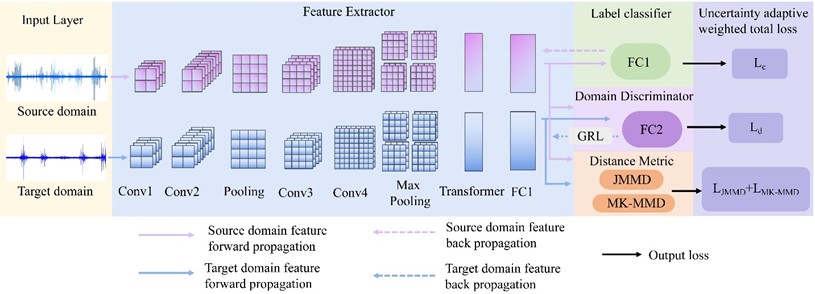
Table 1Pseudo-code of the model

Algorithm: universal domain alignment and multi-level alignment network

Require: Source set

D_{s} = x^{s}

,

y^{s}

, target set

D_{t} = x^{s}

, class number

K

; trade-off weights

λ_{1} λ_{2}

;

Learnable uncertainty scales

σ_{c} σ_{d} σ_{a}

,

σ_{c}^{2}

,

σ_{d}^{2}

,

σ_{a}^{2} > 0

; GRL schedule parameter

γ

Initialize feature extractor

θ_{f}

, classifier

θ_{y}

, domain discriminator

θ_{d}

, learnable logs, training progress

p \leftarrow 0

While not converged do

Sample minibatches

x^{s}

,

y^{s} ~ D_{s}

,

x^{s} ~ D_{t}

Feature extraction:

f_{s}

,

J_{s} \leftarrow G_{f} (x_{s}; θ_{f})

,

f_{t}, J_{t} \leftarrow G_{f} (x_{t}; θ_{f})

Label prediction:

z_{s} \leftarrow G_{y} (f_{s}; θ_{y})

,

L_{c} \leftarrow C r o s s E n t r o p y (Z_{s}, y_{s})

Domain discrimination with GRL:

d_{s} \leftarrow G_{d} (G R L (f_{s}); θ_{d})

,

d_{t} \leftarrow G_{d} (G R L (f_{t}); θ_{d})

,

L_{d} \leftarrow B C E (d_{s}, 0) + B C E (d_{t}, 1)

Multi-level distribution alignment:

D_{J} \leftarrow J M M D (J_{s}, J_{t})

,

D_{M} \leftarrow M K M M D (f_{s}, f_{t})

,

D_{f u s s d i o n} \leftarrow λ_{1} D_{J} + λ_{2} D_{M}

Dynamic adversarial weight (

β_{a d v}

with progress

p \in [0,1]

),

β_{a d v} \leftarrow \frac{2}{1 + e x p (- γ p)} - 1

Uncertainty-weighted total loss:

L_{t o t a l} \leftarrow \frac{L_{c}}{2 σ_{c}^{2}} + \frac{β_{a d b}}{{2 σ}_{d}^{2}} L_{d} + \frac{D_{f u s i o n}}{{2 σ}_{a}^{2}} + l o g σ_{c} + l o g σ_{d} + l o g σ_{a}

One optimization step

θ_{f}, θ_{y}, θ_{d} \leftarrow

Adam Update

\{θ_{f} {, θ}_{y}, θ_{d}\}, {\nabla L}_{t o t a l}

Update training progress:

p \leftarrow

UpdateProgess ()

end while

Return

θ = {θ_{f}, θ_{y}, θ_{d}}

(1) Input layer.

The input layer receives a vibration signal of length $L$ , expressed as:

1

S = \{S_{1}, S_{2}, \dots {, S}_{L}\}, S \in R^{L \times 1},

where each $s_{i}$ denotes the vibration signal value at the $i$ -th sampling point.

(2) Convolution operation.

The convolutional layer is employed for feature learning and local feature extraction. One-dimensional convolution learns features by convolving a kernel with the $j$ -th segmented signal. The input sequence is denoted as $s^{(l - 1)}$ , and it is supposed that the kernel size, kernel weights, and bias of the $l$ -th convolutional layer are $k^{(l)}$ , $ω^{(l)}$ and $b^{(l)}$ , respectively. Then, the output of the convolutional layer can be expressed as:

2

c_{j} = R E L U (\sum_{i = 1}^{k^{(l)}} ω_{i}^{(l)} \times s_{j - k^{(l)}}^{(l - 1)} + b^{(l)}),

where ReLU denotes the nonlinear activation function; $c_{j}$ represents the $j$ -th element of the convolutional output; multi-scale feature extraction is achieved across different layers by adjusting the kernel size $k^{(l)}$ .

(3) Pooling operation.

A max-pooling layer is applied after the convolutional layer to reduce feature dimensionality and prevent overfitting:

3

P_{j} = m a x \{c_{j - k + 1 : j}\},

where $P_{j}$ signifies the pooled feature, and $c_{j - k + 1 : j}$ represents a local segment with window size $k$ ending at position $j$ . In this study, a pooling window size of $k =$ 2 is adopted. It effectively halves the feature length and reduces computational complexity while preserving salient local features during dimensionality reduction, avoiding the loss of fault-related impulsive information caused by excessive pooling [14].

(4) Transformer attention mechanism.

The Transformer model initially demonstrated outstanding performance in the field of natural language processing and has been increasingly introduced into various time-series signal modeling tasks. Its core concept lies in the Multi-Head Self-Attention (MHSA). MHSA captures global dependencies between different positions in a sequence through parallelized attention computations, thereby effectively compensating for the limitations of traditional convolutional or recurrent architectures in long-range dependency modeling [15].

A self-attention mechanism is introduced on the feature map $P_{j} \in R^{L \times d_{p}}$ obtained after convolution and pooling to further capture long-range dependencies across different time steps. Specifically, $L$ denotes the down-sampled sequence length, and $d_{p}$ represents the number of feature channels. In the attention mechanism, the input features are first linearly projected into a query vector $Q$ , a key vector $K$ , and a value vector $V$ , where $Q$ is used to issue queries, $K$ to measure relevance, and $V$ to represent the actual feature information. The attention weights are computed based on the similarity between $Q$ and $K$ and then employed to perform a weighted aggregation over $V$ , enabling dynamic feature aggregation:

4

Q = P W_{Q}, K = P W_{K}, V = P W_{V},

where $W_{Q}$ , $W_{K}$ , $W_{V} \in R^{d_{p} \times d_{k}}$ embody learnable parameter matrices, and $d_{k}$ signifies the internal dimensionality of the attention mechanism.

The self-attention is computed as:

5

A t t e n t i o n (Q, K, V) = s o f t m a x (\frac{Q K^{T}}{\sqrt{d_{k}}}) V .

Under the multi-head attention mechanism, let the number of attention heads be $h$ , and then the $i$ -th attention head is defined as:

6

{h e a d}_{i} = A t t e n t i o n ({Q W}_{Q}^{i}, {K W}_{K}^{i}, {V W}_{V}^{i}) .

After concatenating all attention heads, the output is obtained as:

7

M u l t i H e a d (Q, K, V) = C o n c a t ({h e a d}_{1}, \dots, {h e a d}_{h}) W_{0},

where $W_{0} \in R^{h d_{v} \times d}$ indicates the output projection matrix. The number of heads in the multi-head attention mechanism exerts a significant impact on model performance and is typically set to 2, 4, or 8 in practice. An excessively large number of heads may boost the risk of overfitting and slow down convergence, whereas too few heads may induce underfitting. In this study, the number of attention heads is set to 4 [16], and the dimensionality of each head is defined as $d_{k} = d_{v} = d / 4$ , where $d_{v}$ represents the dimensionality of the value vector in each attention head.

(5) Fully connected layer.

The feature representation $f \in R^{d}$ , obtained from the multi-head attention mechanism is fed into a fully connected layer:

8

f^{'} = σ (W_{f}^{T} f + b_{f}), W_{f} \in R^{d \times d_{f c}},

where $σ (∙)$ denotes the activation function, and the ReLU activation function is adopted in this study; $b_{f}$ represents the bias term; $d_{f c}$ signifies the output dimensionality of the fully connected layer.

(6) Output layer.

Finally, the output layer employs the Softmax function to transform the outputs of the fully connected layer into a probability distribution, enabling fault category classification:

9

y_{c} = \frac{e x p (W_{c}^{T} f^{'} + b_{c})}{\sum_{k = 1}^{K} e x p W_{k}^{T} f^{'} + b_{k})}, c = 1,2, \dots, K,

where $K$ denotes the total number of fault categories; $W_{c}$ and $b_{c}$ are the class-specific weight vector and bias term for class $c$ , respectively; $b_{c}$ represents the bias associated with class $c$ , and $b_{k}$ embodies the bias term corresponding to class kin the summation. The output vector $y = [y_{1}, y_{2} {, ∙ ∙ ∙ y}_{k}]$ provides the predicted probabilities for all fault categories. The final classification result is determined by selecting the category with the maximum probability.

2.2. Domain adaptive module

The domain adaptation module of the proposed model consists of a JMMD-based distance metric, an MK-MMD-based distance metric, and a domain discriminator module.

2.2.1. Feature distribution difference measurement module

Under varying operating conditions, a single distribution alignment method is typically insufficient to simultaneously ensure cross-layer joint distribution consistency and capture multi-scale distribution discrepancies, consequently degrading diagnostic accuracy. Given this issue, JMMD and MK-MMD are integrated in this study. The former constrains the joint distributions of multi-layer features; the latter enhances robustness to discrepancies at different scales through multi-kernel weighting. They jointly curtail feature shifts between the source and target domains in both marginal and conditional distributions. Compared with the conventional single Maximum Mean Discrepancy method, JMMD [17] integrates multi-level feature mappings to more comprehensively characterize and lessen distribution discrepancies across different domains, enabling the optimization of the joint distributions of multiple feature representations and enhancement of feature extraction and domain alignment performance [18].

In the fault identification classifier, deep feature vectors, $f_{1}^{s}$ and $f_{1}^{t}$ , are first extracted from the source and target domains through the feature extraction network. Subsequently, they are further projected into a unified feature space through the fully connected layer FC1. With the purpose of achieving cross-domain distribution alignment, the feature representations of the source and target domains in this space are denoted as $ϕ (f_{1}^{s})$ and $ϕ (f_{1}^{t})$ , respectively, where $ϕ (\cdot)$ embodies a kernel mapping function that projects features into a reproducing kernel Hilbert space (RKHS). JMMD enforces collaborative consistency between the source and target domains across both convolutional features and high-level semantic features, preventing situations in which lower-level features are well aligned while substantial discrepancies remain at higher levels. Thus, discriminative capability can be reinforced under varying operating conditions.

The corresponding formulation is:

10

J M M D (P, Q) = \sum_{l = 1}^{L} {‖E_{f_{1}^{s}} ~ P [ϕ^{(l)} (f_{1}^{s})] - E_{f_{1}^{t}} ~ Q [ϕ^{(l)} (f_{1}^{t})]‖}_{H_{l}}^{2},

where $P$ and $Q$ denote the feature distributions of the source and target domains, respectively; $ϕ^{(l)} (\cdot)$ indicates the feature mapping function of the $l$ -th layer that maps features into a reproducing kernel Hilbert space for computing mean embeddings; $f_{1}^{s}$ , $f_{1}^{t}$ represent the feature representations of the source and target domains; $H_{l}$ embodies the RKHS associated with the $l$ -th layer; ${‖\cdot‖}_{H_{l}}$ refers to the norm defined in the Hilbert space $H_{l}$ .

Multi-kernel Maximum Mean Discrepancy (MK-MMD) [19] indicates an extension of the conventional MMD that further enhances distribution alignment capability. MMD characterizes the distribution discrepancy between the source and target domains by mapping samples into a RKHS and computing the distance between their mean embeddings [20], defined as:

11

d_{k}^{2} (p, q) = {‖E_{f_{1}^{s}} ~ P [ϕ_{k} (f_{1}^{s})] - E_{f_{1}^{t}} ~ Q [ϕ_{k} (f_{1}^{t})]‖}_{H_{l}}^{2},

where $ϕ_{k} (\cdot)$ denotes the feature mapping associated with the $k$ -th kernel function into a RKHS; $H_{k}$ represents the RKHS induced by the $k$ -th kernel; $d_{k}^{2} (p, q) = 0$ and only if the distributions $p$ and $q$ are identical.

In practical applications, the choice of a single kernel function can significantly impact alignment performance. Since MK-MMD constructs multiple kernel functions at different scales and combines them through weighted summation, the model can capture both global and local feature variations when measuring distribution discrepancies. Accordingly, MK-MMD constructs a composite kernel through a non-negative convex combination of multiple kernels:

12

K (f_{1}^{s}, f_{1}^{t}) = \sum_{u = 1}^{m} β_{u} k_{u} (f_{1}^{s}, f_{1}^{t}), s u b j e c t t o \sum_{u = 1}^{m} β_{u} = 1, β_{u \geq 0},

where $k (∙, ∙)$ denotes the $u$ -th base kernel function, $β_{u}$ represents the weight of the $u$ -th kernel, and $m$ denotes the number of kernel functions. This strategy alleviates the sensitivity to single-kernel selection while fully exploiting the advantages of different kernel functions at multiple scales. Therefore, combining Eqs. (10) and (12) yields the resulting distance metric as:

13

\{\begin{matrix} D_{J M M D} = \sum_{l = 1}^{L} {‖E_{f_{1}^{s}} ~ P [ϕ^{(l)} (f_{1}^{s})] - E_{f_{1}^{t}} ~ Q [ϕ^{(l)} (f_{1}^{t})]‖}_{H_{l}}^{2}, \\ D_{M K - M M D} = {‖E_{f_{1}^{s}} ~ P [ϕ_{K} (f_{1}^{s})] - E_{f_{1}^{t}} ~ Q [ϕ_{K} (f_{1}^{t})]‖}_{H_{l}}^{2}, \\ ϕ_{K} (f) = \sum_{i = 1}^{m} α_{i} ϕ_{k_{i}} (f), \sum_{i = 1}^{m} α_{i} = 1, α_{i} \geq 0, \\ D_{f u s s i o n} = λ_{1} D_{J M M D} + λ_{2} D_{M K - M M D}, \end{matrix}

where $L$ denotes the number of feature layers jointly aligned by JMMD; $ϕ_{k_{i}} (f)$ represents the mapping of the feature vector f induced by the $i$ -th base kernel; $ϕ_{K} (f)$ signifies the composite multi-kernel mapping used in MK-MMD; $α_{i}$ refers to the weight of the $i$ -th kernel function; $λ_{1}$ , $λ_{2}$ are the balancing coefficients for integrating JMMD and MK-MMD, respectively. Through the fusion of JMMD and MK-MMD, the model aligns the joint feature distributions between the source and target domains while simultaneously capturing distribution discrepancies at multiple scales, thereby alleviating distribution shift under varying operating conditions.

2.2.2. Domain discriminator

After feature extraction of bearing vibration signals with a convolutional neural network, the feature distributions under different operating conditions may differ significantly. As a result, the features learned from the source condition become difficult to transfer directly to the target condition. Given this issue, a domain discriminator is introduced after the integration of JMMD and MK-MMD, and an adversarial framework is constructed by incorporating a gradient reversal layer (GRL) [21]. The domain discriminator attempts to identify the operating condition from which the input features originate, while the feature extractor is continuously optimized during training to confuse the discriminator. Thus, it learns more domain-invariant feature representations and improves cross-condition fault diagnosis performance.

The domain classifier is primarily composed of two components: a fully connected layer (FC2) and a domain discriminator output layer (DO). These two layers jointly ensure that the network can effectively distinguish data features from different domains.

Fully connected layer FC2: FC2 receives the feature representation $f_{1}$ from FC1 and produces a new feature representation $f_{2}$ through linear transformation and nonlinear activation:

14

f_{2} = σ (W_{f}^{T} f_{1} + b_{f}),

where $f_{1}$ denotes the sigmoid activation function; $W_{f}$ and $b_{f}$ refer to the weight matrix and bias term of this layer, respectively.

Domain discriminator output layer (DO) is a binary classifier specifically designed to distinguish whether the input features belong to the source domain or the target domain. The output of this layer, denoted as $d$ , is given by:

15

d = \frac{1}{1 + e x p (- (W_{d}^{T} f_{2} + b_{f})},

where $W_{d}$ denotes the output weight matrix of the domain discriminator, and $b_{d}$ represents the corresponding bias term. Therefore, the output $d \in (0,1)$ can be interpreted as the probability that the input feature belongs to the source or target domain. Through the adversarial training mechanism, the domain discriminator continuously enhances its capability to distinguish features from different domains. Meanwhile, the feature extractor, under the effect of reversed gradients, gradually learns more domain-invariant feature representations. Consequently, it achieves multi-dimensional alignment of discriminative features, alleviates distribution shift between domains, and effectively reduces cross-domain distribution discrepancies under varying operating conditions.

2.2.3. Definition of loss function

The source domain dataset is denoted as $D_{s} = {\{(x_{i}^{s}, y_{i}^{s})\}}_{i = 1}^{n_{s}}$ , where $x_{i}^{s}$ represents the $i$ -th source-domain input sample, $y_{i}^{s}$ signifies the corresponding label, and $n_{s}$ embodies the number of source-domain samples. Besides, the target domain dataset is defined as $D_{t} = {\{(x_{j}^{t})\}}_{j = 1}^{n_{t}}$ , where $x_{j}^{t}$ and $n_{t}$ refer to the $j$ -th target-domain input sample and the number of target-domain samples, respectively. The feature extractor is denoted as $G_{f} (∙)$ , which is used to extract features from the input data, and its output is defined as $f_{1} (x) = G_{f} (x)$ with the corresponding source-domain and target-domain feature representations given by $f_{1}^{s} = G_{f} (x_{i}^{s})$ , $f_{1}^{t} = G_{f} (x_{j}^{t})$ . The label classifier is denoted as $G_{y} (∙)$ , whose logits output is given by $z (x) = {W_{c}^{T} f}_{1} (x) + b_{c}$ , and the Softmax probability vector is defined as $p (x) = s o f t m a x (z (x))$ .

(1) Classification loss $L_{c}$ : a multi-class cross-entropy loss applied to labeled source-domain samples, which constrains the classification capability of the classifier on the source domain, defined as:

16

L_{c} = - \frac{1}{m} \sum_{i = 1}^{m} \sum_{k = 1}^{K} I [y_{i}^{s} = k] l o g \frac{\exp (W_{c}^{(k) T} f_{1} (x_{i}^{s}) + b_{c}^{(k)})}{\sum_{j = 1}^{K} \exp (W_{c}^{(j) T} f_{1} (x_{i}^{s}) + b_{c}^{(j)})},

where $f_{1} (x_{i}^{s}) = G_{f} (x_{i}^{s}) \in R^{d}$ denotes the feature vector extracted by the feature extractor $G_{f} (\cdot)$ , with dimensionality d; $W_{c} = [W_{c}^{(1)}, \dots, W_{c}^{(k)}] \in R^{d \times K}$ indicates the classifier weight matrix, and $W_{c}^{(k)}$ stands for the weight column vector corresponding to the $k$ -th class; ${b_{c} = [b_{c}^{(1)}, \dots, b_{c}^{(k)}]}^{T}$ represents the bias vector, and each element, $b_{c}^{(k)}$ , corresponds to the bias term of the $k$ -th class; $I (\cdot)$ embodies the indicator function, and $I [y_{i}^{s} = k] = 1$ if $y_{i}^{s} = k$ and 0 otherwise; $K$ signifies the total number of fault categories, and $m$ denotes the mini-batch size of the source domain. The fraction in the formulation is related to the Softmax probability, and the predicted probability of the $k$ -th class $p_{k} (x_{i}^{s})$ is defined as:

17

p_{k} (x_{i}^{s}) = \frac{\exp (W_{c}^{(k) T} f_{1} (x_{i}^{s}) + b_{c}^{(k)})}{\sum_{j = 1}^{K} \exp (W_{c}^{(j) T} f_{1} (x_{i}^{s}) + b_{c}^{(j)})},

where $p_{k} (x_{i}^{s})$ denotes the predicted probability that the input sample $x_{i}^{s}$ belongs to the $k$ -th class.

(2) Domain discrimination loss $L_{d}$ : The domain discrimination loss is employed to guide adversarial training between the feature extractor and the domain discriminator, allowing for the learning of domain-invariant features. Binary cross-entropy loss is computed for both source-domain and target-domain samples through the domain discriminator. The feature extractor and the domain discriminator are jointly optimized in an adversarial manner by computing the binary cross-entropy loss for source and target samples separately. Let $\hat{d} = σ (G_{d} (G R L (F)))$ , and then the loss for a single sample is defined as:

18

l_{d} = (f, d) = - [d l o g \hat{d} + (1 - d) \log (1 - \hat{d})],

where $\hat{d}$ denotes the model output; $d$ represents the domain label, 0 or 1; they correspond to the source domain and the target domain, respectively. Accordingly, the domain discrimination loss $L_{d}$ is defined as the average loss over source-domain and target-domain samples:

19

L_{d} = \frac{1}{n_{s}} \sum_{i = 1}^{n_{s}} L_{d} (f_{1}^{s_{i}}, 0) + \frac{1}{n_{t}} \sum_{j = 1}^{n_{t}} L_{d} (f_{1}^{s_{j}}, 1),

where $f_{1}^{s_{i}}$ and $f_{1}^{s_{j}}$ represent the feature vectors of the source-domain and target-domain samples, respectively, extracted by the feature extractor $G_{f}$ ; $L_{d} (∙)$ denotes the binary cross-entropy loss for a single sample, measuring the discrepancy between the domain discriminator output $\hat{d}$ and the domain label $d$ ; $n_{s}$ , $n_{t}$ signify the numbers of samples in the source and target domains, respectively; $G_{d}$ indicates the domain discriminator, which aims to distinguish whether a sample belongs to the source or target domain by minimizing the loss $L_{d}$ during training; GRL stands for the gradient reversal layer, which reverses the gradient propagated to the feature extractor $G_{f}$ during backpropagation, thereby encouraging $G_{f}$ to learn domain-invariant feature representations.

(3) Distribution distance loss $D_{f u s i o n}$ : With the purpose of further aligning the feature distributions between the source and target domains, the JMMD and MK-MMD losses are integrated into a unified metric for measuring the discrepancy between the joint feature distributions of the source and target domains. Through this fusion, the model can align multi-level feature distributions between the source and target domains while simultaneously capturing distribution discrepancies at multiple scales, thereby alleviating distribution shift stemming from varying operating conditions. According to Eq. (13), the final fused loss is defined as:

20

D_{f u s i o n} = λ_{1} D_{J M M D} + λ_{2} D_{M K - M M D},

where $D_{J M M D}$ and $D_{M K - M M D}$ denote the JMMD and MK-MMD loss terms, respectively; $λ_{1}$ , $λ_{2}$ control the relative weights of the two metrics.

(4) Uncertainty-Adaptive Weighted Overall Loss: An uncertainty-based adaptive weighting strategy is introduced [22] to avoid manual hyperparameter tuning. Specifically, three objectives, namely the classification loss $L_{c}$ , the domain discrimination loss $L_{d}$ , and the distribution distance loss $D_{f u s i o n}$ , are each associated with a learnable uncertainty scale satisfying $σ_{c}^{2}$ , $σ_{d}^{2}$ , $σ_{a}^{2} > 0$ . The model is trained by minimizing the total loss $L_{t o t a l}$ to jointly improve domain adaptation and classification accuracy. The overall loss is defined as:

21

L_{t o t a l} = \frac{1}{2 σ_{c}^{2}} L_{c} + \frac{β_{a d b}}{{2 σ}_{d}^{2}} L_{d} + \frac{1}{{2 σ}_{a}^{2}} D_{f u s i o n} + l o g σ_{c} + l o g σ_{d} + l o g σ_{a}

where $σ_{c}^{2}$ , $σ_{d}^{2}$ and $σ_{a}^{2}$ are learnable variances associated with the classification loss, domain discrimination loss, and distribution alignment loss, respectively; $l o g σ_{d}$ , $l o g σ_{a}$ , $l o g σ_{c}$ denote regularization terms that constrain the magnitude of the variances and prevent excessive adjustment; $β_{a d v}$ represents the adversarial training strength, with $β_{a d v} \in (0,1]$ , which is progressively increased with the training progress $p \in [0,1]$ following $β_{a d v} = \frac{2}{1 + e x p (- γ p)} - 1$ to stabilize adversarial training

3. Test verification and result analysis

3.1. Western Reserve University data validation

The rolling bearing vibration signal dataset used in this study was obtained from the Electrical Engineering Laboratory of Case Western Reserve University (CWRU), USA [23]. During the experiments, the vibration signals of rolling bearings were recorded as multivariate vibration time series and collected by a data acquisition system at sampling frequencies of 12 kHz and 48 kHz, among which the 12 kHz sampling frequency was adopted in this work. Rolling bearing datasets under four operating conditions were obtained as per different combinations of rotational speed and load. Each operating condition in the CWRU dataset includes four bearing states: normal (N), inner race fault (IF), outer race fault (OF), and ball fault (BF), as detailed in Table 2. Considering both bearing condition and fault size, each operating condition contains ten bearing states: N, IF18, BF18, OF18, IF36, BF36, OF36, IF54, BF54, and OF54. Concerning data preparation, the signals were segmented into approximately 100 samples per class, with each sample having a length of 1024 points. With respect to each operating condition, 80 % of the samples were employed for training and the remaining 20 % for testing. Additionally, the number of training epochs was set to 99, the Adam optimizer was applied, the initial learning rate was set to 0.001, and the batch size was set to 64.

Table 2Specific data of working conditions

Condition / domain	revolution speed (r/min)	Load (HP)	Fault size
0hp	1797	0	0.1778 0.3556 0.5334
1hp	1772	1
2hp	1750	2
3hp	1730	3

3.1.1. Different training batch tests

Under varying operating conditions, the batch size setting influences the estimation accuracy of alignment losses, the convergence behavior of distribution distances between the source and target domains, and the stability of domain adversarial training. Thus, comparative experiments were conducted on the proposed UDAM-Net model across ten transfer tasks to investigate this influence, and the average results were reported. The batch size was set to 32, 50, 64, 90, and 128, respectively. The experimental results are summarized in Table 3.

Table 3Average experimental results of different training batches of 10 migration tasks

Batch	Accuracy	Precision	Recall	F1-score
32	95.16 %	94.00 %	95.00 %	94.50 %
50	94.33 %	90.66 %	92.00 %	90.67 %
64	96.67 %	96.67 %	96.00 %	96.00 %
90	96.33 %	96.33 %	96.00 %	96.00 %
128	95.83 %	95.17 %	95.75 %	95.46 %

As observed from Table 3, the UDAM-Net model achieves its best performance when the batch size is set to 64. Across the 12 transfer tasks, the average diagnostic accuracy, precision, recall, and F1-score reach 96.67 %, 96.67 %, 96 %, and 96 %, respectively, all of which are higher than those obtained with the other four batch sizes. Thus, the training batch size is uniformly set to 64 in all subsequent experiments, ensuring model stability and optimal performance.

3.1.2. Contrast test

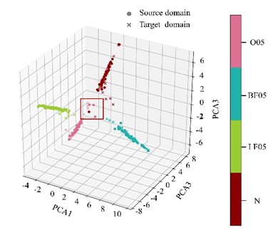
Comparative experiments were conducted to verify the effectiveness of the proposed UDAM-Net in reducing the feature distribution discrepancy between the source and target domains under variable operating conditions. The UDAM-Net model was compared with 1DCNN-Transformer, CORAL, KL divergence, Proxy-A distance, as well as the existing methods CNN-BiLSTM-Transformer [24] and CNN-MDD [25]. The performance was evaluated through four metrics: accuracy, precision, recall, and F1-score. The results, averaged over 12 transfer tasks, are summarized in Table 4. With the 1 hp to 2 hp operating condition as an example, Fig. 2(a) illustrates PCA-based feature clustering, where high-dimensional features are projected into a three-dimensional space for visualization. Fig. 2(b) exhibits the corresponding confusion matrix. Table 4 lists the averaged experimental results.

As illustrated in Fig. 2(a), the distribution discrepancy between the source and target domain features has been largely reduced, with only a small portion of features failing to fully overlap. Fig. 2(b) reflects that 4.17 % of IF36 samples are misclassified as IF18, and BF53 samples are misclassified as IF53, while all other fault types are correctly identified. As revealed from Table 4, UDAM-Net outperforms the other methods across all four evaluation metrics. Compared with the baseline models CNN-BiLSTM-Transformer and CNN-MDD, UDAM-Net achieves accuracy improvements of 3.16 % and 6.41 %, respectively, demonstrating its advantage in achieving higher diagnostic accuracy.

Fig. 2Fig. 5(a) Feature clustering results and confusion matrix

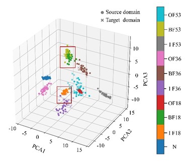
a) Feature clustering results

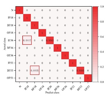
b) Confusion matrix

Table 4Comparison of model index results

	Accuracy	Precision	Recall	F1-Score
1DCNN-Transformer	93.75 %	93.41 %	91.89 %	92.65 %
CORAL	94.00 %	93.75 %	93.08 %	93.42 %
KL	73.83 %	79.00 %	72.75 %	75.88 %
Proxy a distance	90.10 %	92.34 %	87.67 %	90.01 %
CNN-BiLSTM-Transformer	93.51 %	90.00 %	93.00 %	91.50 %
CNN-MDD	90.26 %	94.00 %	91.00 %	92.50 %
UDAM-Net	96.67 %	96.67 %	96.00 %	96.34 %

3.1.3. Ablation test

The effects of 1DCNN-Transformer, JMMD, MK-MMD, JMMD–MK-MMD, and UDAM-Net without the Transformer layer (denoted as UDAM-Net (none)) on overall model performance were investigated to evaluate the adaptability of different modules in the proposed model under variable operating conditions and their contributions to fault diagnosis performance. The performance is evaluated with accuracy, precision, recall, and F1-score. The experimental results are presented in Table 5.

Table 5Comparison results of the ablation test model indexes

	Accuracy	Precision	Recall	F1-score
1DCNN-Transformer	92.33 %	92.99 %	92.08 %	92.54 %
JMMD	93.75 %	93.41 %	91.89 %	91.83 %
MKMMD	94.08 %	93.58 %	94.00 %	93.79 %
JMMD-MK-MMD	95.83 %	95.33 %	95.75 %	95.54 %
UDAM-Net	96.67 %	96.67 %	96.00 %	96.00 %
UDAM-Net(none)	89.67 %	89.00 %	88.50 %	88.75 %

As suggested in Table 5, the model accuracy increases by 1.42 % and 1.75 % after the introduction of JMMD and MK-MMD, respectively. The accuracy improvement reaches 3.5 % when the two metrics are combined. Furthermore, the model accuracy is further improved to 96.67 % after the introduction of the domain discriminator. In contrast, removing the Transformer layer yields a significant accuracy decrease of 7 %, specifying the importance of the Transformer-based self-attention mechanism for feature extraction under complex operating conditions. Thus, the 1D-CNN, JMMD–MK-MMD, domain discriminator, and Transformer modules play critical roles in enhancing overall model performance.

3.1.4. Optimizer comparison test

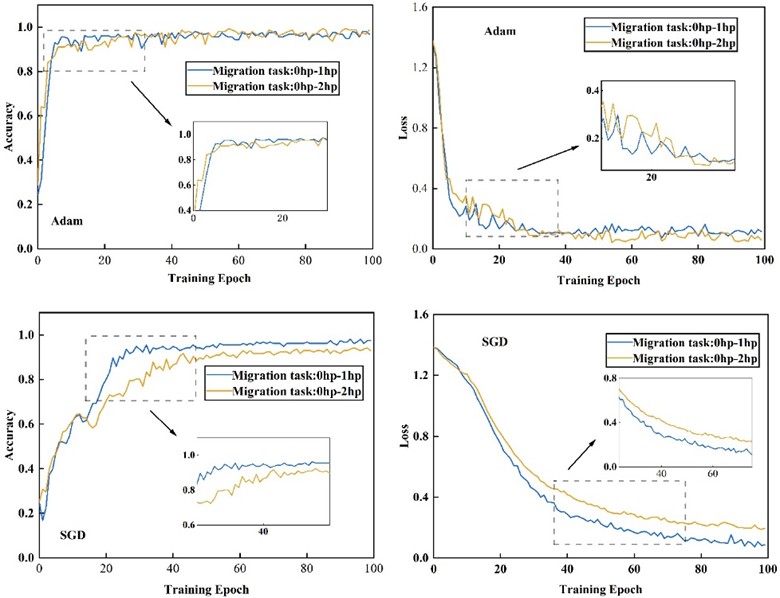
An optimizer comparison experiment was conducted to address the challenges of accelerating model convergence, improving training stability, and avoiding local optima under varying operating conditions. Considering the effects of distribution discrepancy and gradient fluctuations during training, Adam and SGD optimizers were selected for comparison, with the learning rate set to 0.001 for both. Among the 12 transfer tasks, three representative tasks (1 hp to 2 hp, 1 hp to 3 hp, and 2 hp to 1 hp) were selected as examples to evaluate their effects on model convergence speed, training stability, and final transfer capability. The corresponding accuracy and loss curves are illustrated in Fig. 3.

Fig. 3Optimizer sparrow rate and loss rate comparison

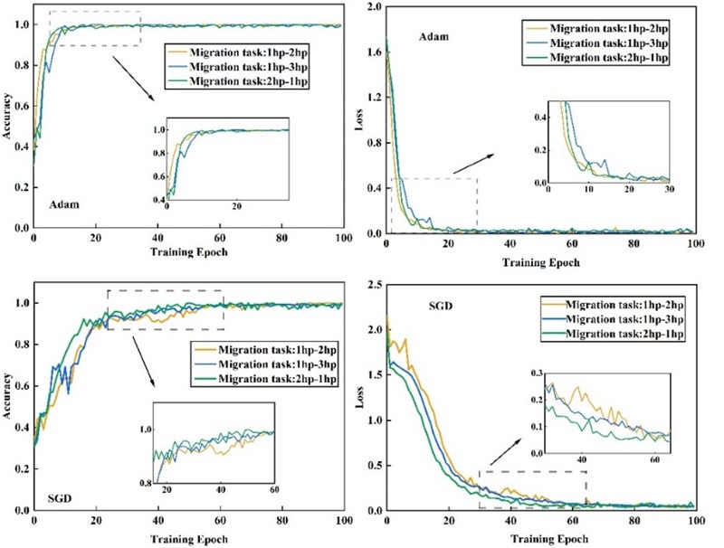
Fig. 5 reveals that, for the selected transfer tasks, the model optimized with Adam achieves stable accuracy and loss values after approximately 20 iterations. In contrast, the model using the SGD optimizer requires nearly 60 iterations to reach convergence. To sum up, the Adam optimizer outperforms SGD in convergence speed and stability under varying operating conditions, making it more suitable for the proposed UDAM-Net model.

3.2. Fault test bench test verification

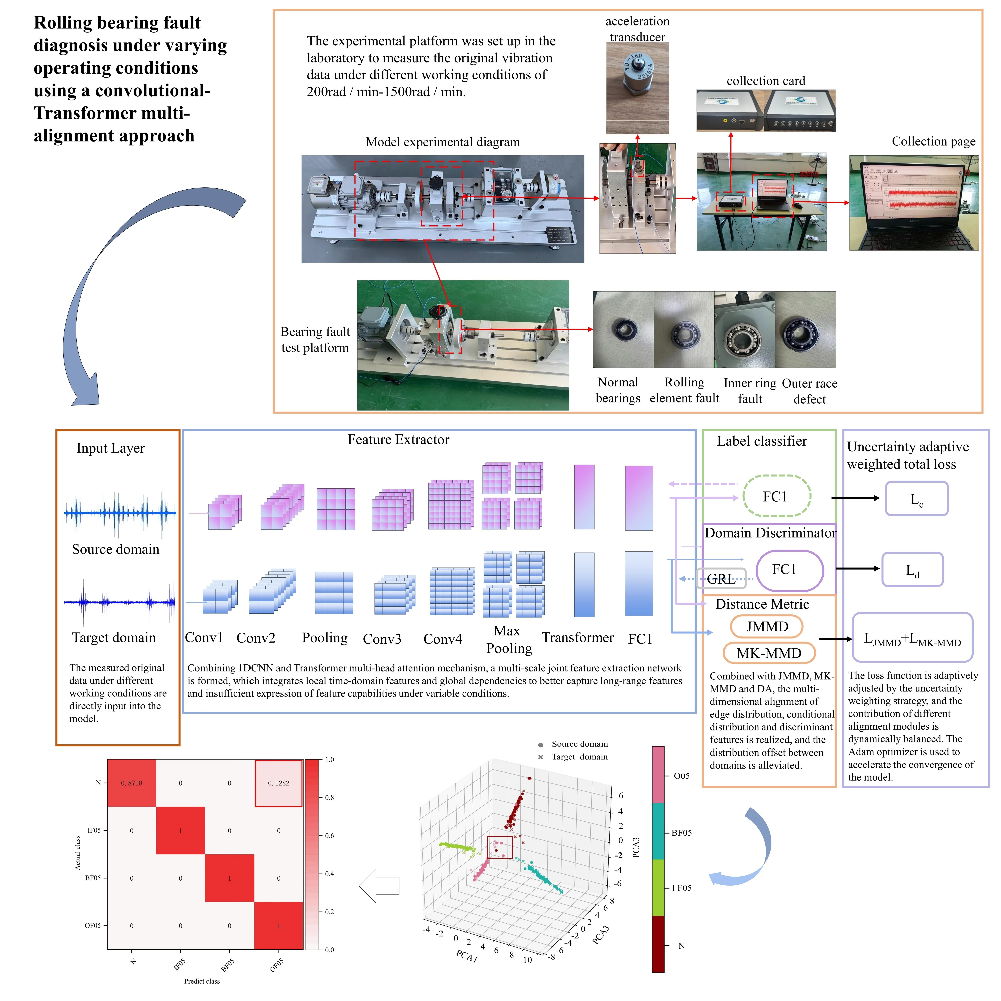
Experiments were conducted with data collected from a laboratory-built test rig to verify the feasibility and generalization capability of the proposed model in practical applications. The bearing fault experimental setup is illustrated in Fig. 4. The fault categories and corresponding parameters are detailed in Tables 6 and 7. The test ring mainly consists of accelerometers, a data acquisition card, a data acquisition system, and a speed controller. Two experiments were conducted in this study. During the experiments, accelerometers 1, 2, and 3 correspond to channels ch01, ch02, and ch03 in the acquired CSV files, respectively. The data from channel ch02 were selected for analysis. The data acquisition unit employs a 24-bit ADC with eight vibration and voltage channels, supporting a maximum sampling frequency of 77.16 kHz per channel, along with an additional speed channel. It is equipped with a front-end Butterworth low-pass filter, bringing about a measurement error below 0.4 %. The data acquisition software provides three gain levels and supports data acquisition, visualization, storage, and analysis. The acquisition parameters are set with a sampling frequency of 77.16 kHz and a sampling duration of approximately 20 s, as well as a load range of 0-100 kg and a rotational speed range of 200-1500 r/min. The tested fault types comprise outer race faults and rolling element faults. After data segmentation, approximately 1500 samples are obtained, each with a length of 1024 points, of which 80 % are adopted for training and 20 % for testing. Additionally, six variable operating condition fault diagnosis tasks are constructed based on the four bearing fault categories in Table 6 and the three operating conditions in Table 7. The experimental settings are consistent with those of the Case Western Reserve University dataset. Comparative experiments, ablation studies, and optimizer comparison experiments are conducted. The experimental results are evaluated with accuracy, precision, recall, and F1-score. The photograph of the experimental platform in Fig. 4 was taken by the laboratory team at Room 305, School of Mechanical and Equipment Engineering, Hebei University of Engineering, on August 23, 2024.

Fig. 4The main components of the test bench

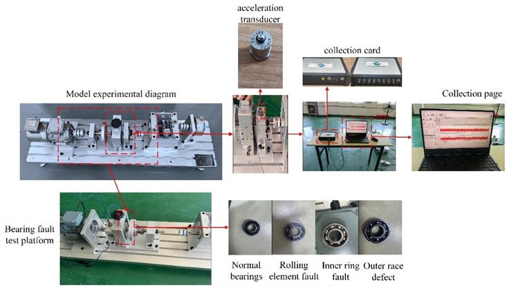
Table 6Classification of bearing state

Fault category	Numbering	Fault state	Degree of injury /mm
1	N00	normal state	0
2	IF05	Rolling element fault	0.5
3	BF05	Inner ring fault	0.5
4	OF05	outer race defect	0.5

Table 7Test condition parameters

Condition / domain	revolution speed (r/min)	Load (HP)
0 hp	800	25%
1 hp	900	50%
2 hp	1000	100%

3.2.1. Comparative test of the fault test bench

Comparative models consistent with those used in the Case Western Reserve University experiments are adopted in this section to verify the effectiveness of the proposed method. The evaluation is performed by calculating the average accuracy, precision, recall, and F1-score across six different transfer tasks. With the 2 hp to 0 hp transfer task as an example, the feature clustering results and confusion matrix of the proposed model are presented in Fig. 5(a) and Fig. 5(b), respectively. The averaged evaluation metrics are summarized in Table 8. The classification accuracies of the seven models across the six transfer tasks are detailed in Table 9.

Fig. 5Feature clustering results and 1DCNN-UDAM-Net confusion matrix

a) Feature clustering results

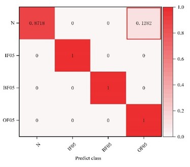
b) 1DCNN-UDAM-Net confusion matrix

Table 8Test bench comparison test model diagnosis results

	Accuracy	Precision	Recall	F1-score
1DCNN-Transformer	80.33 %	77.67 %	82.00 %	79.84 %
CORAL	80.00 %	81.67 %	80.00 %	80.84 %
KL	71.00 %	72.17 %	71.00 %	71.59 %
Proxy a distance	86.83 %	86.70 %	86.80 %	86.75 %
CNN-BiLSTM-Transformer	90.83 %	89.33 %	86.67 %	88.01 %
CNN-MDD	86.17 %	83.00 %	83.00 %	83.00 %
UDAM-Net	96.16 %	96.00 %	95.50 %	95.75 %

Table 9Accuracy of different model migration tasks

	0 hp-1 hp	0 hp-2 hp	1 hp-0 hp	1 hp-2 hp	2 hp-0 hp	2 hp-1 hp
1DCNN-Transformer	96.00 %	75.00 %	84.00 %	81.00 %	72.00 %	74.00 %
CORAL	93.00 %	71.00 %	91.00 %	72.00 %	62.00 %	91.00 %
KL	72.00 %	76.00 %	82.00 %	78.00 %	49.00 %	69.00 %
Proxy a Distance	97.00 %	75.00 %	92.00 %	89.00 %	83.00 %	85.00 %
CNN-BiLSTM-Transformer	93.00 %	92.00 %	86.00 %	96.00 %	86.00 %	92.00 %
CNN-MDD	86.00 %	94.00 %	77.00 %	78.00 %	93.00 %	89.00 %
UDAM-Net	98.00 %	92.00 %	99.00 %	97.00 %	95.00 %	96.00 %

As observed from Fig. 5(a), for the 1 hp to 2 hp transfer task, the feature distribution discrepancy between the source and target domains is not fully overlapped only for the outer race fault and normal conditions. Fig. 5(b) suggests that 12.82 % of normal bearing samples are misclassified as outer race faults, while all other fault types are correctly identified. As reported in Table 8, UDAM-Net outperforms the other metric-based methods and baseline models across all four evaluation metrics. Table 9 reflects that, particularly for the 0 hp to 2 hp task, the proposed model achieves accuracy comparable to that of ResNet-DANN and 1DCNN-DANN, with a slight decrease. Nonetheless, the proposed model consistently outperforms the competing methods under the other operating conditions, achieving the best overall performance.

3.2.2. Failure test bench ablation test

With the purpose of evaluating the overall effectiveness of each metric module under practical operating conditions, ablation experiments were conducted on a laboratory-built experimental platform to further validate the generalization and feasibility of the proposed model. The ablation models adopted in this experiment are consistent with those used in the Case Western Reserve University experiments. The averaged results are summarized in Table 10. The experimental results under six operating conditions are detailed in Table 11.

Table 10Comparison of diagnostic results of ablation test model indexes on the test bench

	Accuracy	Precision	Recall	F1-score
1DCNN- Transformer	80.33 %	77.67 %	82.00 %	79.84 %
JMMD	88.50 %	89.67 %	89.00 %	89.34 %
MKMMD	89.83 %	91.83 %	91.00 %	91.42 %
JMMD-MK-MMD	92.33 %	90.50 %	90.67 %	90.59 %
UDAM-Net	96.16 %	96.00 %	95.50 %	95.75 %
UDAM-Net(none)	76.50 %	75.67 %	75.50 %	75.59 %

Table 11Diagnostic results of the migration task of the ablation test model on the test bench

	0 hp-1 hp	0 hp-2 hp	1 hp-0 hp	1 hp-2 hp	2 hp-0 hp	2 hp-1 hp
1DCNN- Transformer	96.00 %	75.00 %	84.00 %	81.00 %	72.00 %	74.00 %
JMMD	94.00 %	83.00 %	95.00 %	84.00 %	83.00 %	92.00 %
MK-MMD	92.00 %	79.00 %	94.00 %	92.00 %	92.00 %	90.00 %
JMMD-MK-MMD	95.00 %	83.00 %	96.00 %	97.00 %	87.00 %	96.00 %
UDAM-Net	98.00 %	92.00 %	99.00 %	97.00 %	95.00 %	96.00 %
UDAM-Net(none)	94.00 %	71.00 %	79.00 %	68.00 %	77.00 %	70.00 %

As revealed in Table 10, the model accuracy reaches 96.16 % after the introduction of JMMD, MK-MMD, and the domain discriminator. In contrast, removing the Transformer layer leads to a significant accuracy decrease of 19.66 %. In other words, the Transformer-based self-attention mechanism substantially enhances feature extraction capability on top of the 1D-CNN backbone. Table 11 reflects that, under the 1 hp to 0 hp and 2 hp to 0 hp operating conditions, introducing the metric modules on top of the 1DCNN-Transformer increases the accuracy by 15 % and 23 %, respectively. Conversely, removing the Transformer layer yields accuracy reductions of 20 % and 18 %, respectively. These results further verify the critical roles of each module in improving overall model performance.

3.2.3. Optimizer comparison test

Experiments are conducted on data collected from the bearing fault test rig to verify the advantage of the Adam optimizer. Specifically, the performance of Adam and SGD was evaluated across six transfer tasks, with the 0 hp to 1 hp and 0 hp to 2 hp operating conditions selected as representative examples. The accuracy and loss curves of the two optimizers under different tasks are illustrated in Fig. 6.

When the Adam optimizer is employed, the model’s accuracy and loss values tend to stabilize after approximately 40 iterations, whereas the SGD optimizer requires around 60 iterations to reach convergence, as suggested in Fig. 6. These results specify that the Adam optimizer exhibits higher convergence efficiency and stability in the 1DCNN-UDAM-Net model, further confirming its advantage in terms of convergence speed and training stability.

Fig. 6Comparison of accuracy and loss rate of self-built test bench optimizer

4. Conclusions

In this study, a deep transfer learning approach that integrates a multi-head attention mechanism with explicit and implicit distance metric learning was established to overcome the challenges of directly extracting discriminative features from raw signals under complex operating conditions, as well as the reduced diagnostic accuracy stemming from cross-domain data distribution imbalance under variable operating conditions. The contribution of each module to the overall framework is systematically validated by comparing the performance of different models. Experimental results demonstrate that, under identical parameter settings, UDAM-Net achieves superior fault diagnosis accuracy and maintains consistent effectiveness across different datasets.

1) The feature extraction capability is significantly enhanced by building upon a 1D-CNN architecture and incorporating a Transformer layer. Additionally, both marginal and conditional distribution alignment capabilities are improved by introducing JMMD and MK-MMD metrics together with a domain discriminator, contributing to the formation of a cross-domain feature alignment framework that combines class discriminability with multi-scale global feature alignment. An uncertainty-based adaptive weighting mechanism is employed to dynamically balance the contributions of different loss terms, thereby reducing the complexity of hyperparameter tuning and significantly enhancing model robustness and cross-domain generalization ability. Finally, the Adam optimizer is adopted to accelerate convergence and improve training stability.

2) The performance of UDAM-Net is validated on both the public CWRU dataset and a self-built experimental platform dataset. Experimental results specify that UDAM-Net achieves average accuracy improvements of 2.67 %, 22.84 %, and 6.57 % over CORAL, KL divergence, and Proxy-A distance, respectively, on the CWRU dataset. Compared with the baseline models CNN-BiLSTM-Transformer and CNN-MDD, further improvements of 3.16 % and 6.41 % are obtained, respectively. Under the operating conditions of the self-built experimental platform, UDAM-Net improves the average accuracy by 13 % and 9 % for the 1 hp to 0 hp and 2 hp to 0 hp transfer tasks, respectively, compared with CNN-BiLSTM-Transformer. In comparison with CNN-MDD, UDAM-Net achieves accuracy improvements of 22 % and 19 % for the 1 hp to 0 hp and 1 hp to 2 hp tasks, respectively. These results further confirm the high diagnostic accuracy of UDAM-Net under practical operating conditions and its superiority across multiple datasets and application scenarios.

3) In the ablation experiments conducted on the CWRU dataset, introducing JMMD and MK-MMD on top of the 1DCNN-Transformer yields an improvement of the accuracy of 1.42 % and 1.75 %, respectively, while their combination brings about an accuracy improvement of 3.5 %. Thus, enhanced feature distribution alignment strengthens cross-domain adaptability. After the introduction of the domain discriminator, the model accuracy is further increased to 96.67 %. This result suggests that the domain discriminator effectively optimizes feature alignment between the source and target domains, reduces inter-domain discrepancies, and enhances adaptability and generalization under variable operating conditions and cross-domain tasks. In contrast, removing the Transformer layer leads to a 7 % decrease in accuracy, further validating the critical role of the Transformer-based self-attention mechanism in feature extraction and long-range dependency modeling. In the ablation experiments conducted on the laboratory-built experimental platform, particularly under the 1 hp to 2 hp and 2 hp to 0 hp operating conditions, introducing the three metric modules into the 1DCNN-Transformer increases the accuracy by 15 % and 23 %, respectively; removing the Transformer layer results in accuracy reductions of 29 % and 18 %, respectively. These results validate that the Transformer self-attention mechanism, the combined JMMD-MK-MMD metrics, and the domain discriminator make critical contributions to performance improvement, enabling UDAM-Net to achieve higher diagnostic accuracy and stronger adaptability under complex operating conditions and cross-domain tasks.

4) The impact of different optimizers on model convergence speed and training stability is evaluated. The results from the experiments conducted on both the CWRU dataset and the self-built dataset unveil that the Adam optimizer achieves rapid convergence and stabilizes after approximately 20 and 40 iterations, respectively, whereas the SGD optimizer requires around 60 iterations to reach a stable state. These findings highlight the clear advantage of the Adam optimizer in accelerating convergence and improving model stability.

5) In future work, the performance of the proposed model will be further investigated under more complex operating conditions, particularly in multi-source domain scenarios involving multiple operating states. Furthermore, its generalization ability and high-accuracy diagnostic performance will be evaluated in situations with limited or missing samples.

References

G.  Yang, W.  Xu, Q.  Deng, Y.  Wei, and F.  Li, “A review of rolling bearing compound fault diagnosis based on vibration signals,” (in Chinese), Journal of Xihua University, Vol. 43, pp. 48–69, 2024, https://doi.org/10.12198/j.issn.1673-159x.5096

Publisher
J. Wang, Z. Xu, W. Liu, Y. Wang, and L. Liu, “Research on health monitoring and fault diagnosis mechanism of rolling bearings,” (in Chinese), Journal of Frontier of Computer Science and Technology, Vol. 18, No. 4, pp. 878–898, 2024.

Search CrossRef
M. Demetgul, K. Yildiz, S. Taskin, I. N. Tansel, and O. Yazicioglu, “Fault diagnosis on material handling system using feature selection and data mining techniques,” Measurement, Vol. 55, pp. 15–24, Sep. 2014, https://doi.org/10.1016/j.measurement.2014.04.037

Publisher
M. Dou, Y. Zhang, F. Sun, and H. Pei, “Combined model: CEEMDAN and AVMD quadratic decomposition noise reduction and BiLSTM-BP classification model rolling bearing fault diagnosis,” Engineering Research Express, Vol. 7, No. 3, p. 035560, Sep. 2025, https://doi.org/10.1088/2631-8695/adfe38

Publisher
X. He, “Research on bearing fault diagnosis based on the fusion of CNN and LSTM algorithms,” in Journal of Physics: Conference Series, Vol. 3057, No. 1, p. 012054, Jul. 2025, https://doi.org/10.1088/1742-6596/3057/1/012054

Publisher
G. Xu, J. Cao, W. Liu, D. Song, J. Zhong, and L. Meng, “Anovel fault diagnosis method for rolling bearing based on SGMD and improved CNN-LSTM,” Engineering Research Express, Vol. 7, No. 3, p. 035567, Sep. 2025, https://doi.org/10.1088/2631-8695/adf93b

Publisher
J. Zou, W. Qiu, Z. Liu, J. Su, T. Chen, and Q. Liu, “Fault diagnosis method for rotating machinery based on FFT-CNN-transformer-crossattention,” International Journal of High Speed Electronics and Systems, Aug. 2025, https://doi.org/10.1142/s0129156425408927

Publisher
X. Shao and C.-S. Kim, “Multi-branch global Transformer‐assisted network for fault diagnosis,” Applied Soft Computing, Vol. 182, p. 113572, Oct. 2025, https://doi.org/10.1016/j.asoc.2025.113572

Publisher
J.  Hu, “Intelligent fault diagnosis of rolling bearings based on VMD-CNN-transformer,” World Journal of Engineering Research, Vol. 3, No. 2, Jan. 2025, https://doi.org/10.61784/wjer3029

Publisher
I. Goodfellow et al., “Generative adversarial networks,” Communications of the ACM, Vol. 63, No. 11, pp. 139–144, Oct. 2020, https://doi.org/10.1145/3422622

Publisher
X. Li, P. Yuan, K. Su, D. Li, Z. Xie, and X. Kong, “Innovative integration of multi-scale residual networks and MK-MMD for enhanced feature representation in fault diagnosis,” Measurement Science and Technology, Vol. 35, No. 8, p. 086108, Aug. 2024, https://doi.org/10.1088/1361-6501/ad4380

Publisher
L. Wan, Y. Li, K. Chen, K. Gong, and C. Li, “A novel deep convolution multi-adversarial domain adaptation model for rolling bearing fault diagnosis,” Measurement, Vol. 191, p. 110752, Mar. 2022, https://doi.org/10.1016/j.measurement.2022.110752

Publisher
H. Wu, J. Li, Q. Zhang, J. Tao, and Z. Meng, “Intelligent fault diagnosis of rolling bearings under varying operating conditions based on domain-adversarial neural network and attention mechanism,” ISA Transactions, Vol. 130, pp. 477–489, Nov. 2022, https://doi.org/10.1016/j.isatra.2022.04.026

Publisher
Y. Tian and X. Liu, “A deep adaptive learning method for rolling bearing fault diagnosis using immunity,” Tsinghua Science and Technology, Vol. 24, No. 6, pp. 750–762, Dec. 2019, https://doi.org/10.26599/tst.2018.9010144

Publisher
G. Xiao, J. Yao, L. Zhong, Z. Xiao, and J. Lu, “MB-ViT: MBConv vision transformer with time-frequency feature fusion for bearing fault diagnosis,” Neural Computing and Applications, Vol. 37, No. 27, pp. 22801–22825, Aug. 2025, https://doi.org/10.1007/s00521-025-11509-7

Publisher
Y. Jin, L. Hou, and Y. Chen, “A Time Series Transformer based method for the rotating machinery fault diagnosis,” Neurocomputing, Vol. 494, pp. 379–395, Jul. 2022, https://doi.org/10.1016/j.neucom.2022.04.111

Publisher
M. Long, H. Zhu, J. Wang, and M. I. Jordan, “Deep transfer learning with joint adaptation networks,” in Proceedings of the 34th International Conference on Machine Learning (ICML 2017), Proceedings of Machine Learning Research, Vol. 70, pp. 2208–2217, 2017.

Search CrossRef
Y. Gao and X. Li, “Fault diagnosis of centrifugal fan bearings based on I-CNN and JMMD in the context of sample imbalance,” Eksploatacja i Niezawodność – Maintenance and Reliability, Vol. 26, No. 4, Jul. 2024, https://doi.org/10.17531/ein/191459

Publisher
G.  Y.  Ganin et al., “Domain adversarial training of neural networks,” Journal of Machine Learning Research, Vol. 17, No. 59, 2016.

Search CrossRef
J. Li, Z. Ye, J. Gao, Z. Meng, K. Tong, and S. Yu, “Fault transfer diagnosis of rolling bearings across different devices via multi-domain information fusion and multi-kernel maximum mean discrepancy,” Applied Soft Computing, Vol. 159, p. 111620, Jul. 2024, https://doi.org/10.1016/j.asoc.2024.111620

Publisher
X. Li et al., “Research on unsupervised domain adaptive bearing fault diagnosis method based on migration learning using MSACNN-IJMMD-DANN,” Machines, Vol. 13, No. 7, p. 618, Jul. 2025, https://doi.org/10.3390/machines13070618

Publisher
Z. Wang et al., “Weighted joint maximum mean discrepancy enabled multi-source-multi-target unsupervised domain adaptation fault diagnosis,” arXiv:2310.14790, Jan. 2023, https://doi.org/10.48550/arxiv.2310.14790

Publisher
W. A. Smith and R. B. Randall, “Rolling element bearing diagnostics using the Case Western Reserve University data: A benchmark study,” Mechanical Systems and Signal Processing, Vol. 64-65, pp. 100–131, Dec. 2015, https://doi.org/10.1016/j.ymssp.2015.04.021

Publisher
X. Yuan and W. Wu, “A bearing fault diagnosis method based on fusion of CNN-BiLSTM-transformer and cross-attention,” Academic Journal of Science and Technology, Vol. 14, No. 2, pp. 191–199, Mar. 2025, https://doi.org/10.54097/594q8441

Publisher
C. Wang, S. Wu, and X. Shao, “Unsupervised domain adaptive bearing fault diagnosis based on maximum domain discrepancy,” EURASIP Journal on Advances in Signal Processing, Vol. 2024, No. 1, pp. 1–12, Jan. 2024, https://doi.org/10.1186/s13634-023-01107-x

Publisher

About this article

Received

September 26, 2025

Accepted

December 28, 2025

Published

February 21, 2026

SUBJECTS

Fault diagnosis based on vibration signal analysis

DOI

https://doi.org/10.21595/jve.2025.25460

Keywords

rolling bearing fault diagnosis

one-dimensional convolutional neural network

joint maximum mean discrepancy

multi-kernel maximum mean discrepancy

domain discriminator

transformer multi-head attention mechanism

Acknowledgements

This work was supported by the Science Research Project of the Hebei Education Department (No. CXY2023002).

Data Availability

The datasets generated during and/or analyzed during the current study are available from the corresponding author on reasonable request.

Author Contributions

Yiying Wang: conceptualization, investigation, methodology, writing-original draft, writing-review and editing, validation, funding acquisition. Fulu Sui: conceptualization, supervision, project administration, formal analysis, data curation. Xiaoling Li: supervision, project administration. Xiaoxin Zhang: conceptualization, funding acquisition, supervision. Mingxian Liu: conceptualization, project administration. Chen Liu: supervision, project administration. Jie Wu: conceptualization, supervision.

Conflict of interest

The authors declare that they have no conflict of interest.

This is an open access article distributed under the Creative Commons Attribution License, which permits unrestricted use, distribution, and reproduction in any medium, provided the original work is properly cited.

Y. Wang et al., “Rolling bearing fault diagnosis under varying operating conditions using a convolutional-Transformer multi-alignment approach,” Journal of Vibroengineering, Vol. 28, No. 2, –20, Feb. 2026, https://doi.org/10.21595/jve.2025.25460

Copy Extrica

Copied to clipboard!

TY  - JOUR
DO  - 10.21595/jve.2025.25460
UR  - https://doi.org/10.21595/jve.2025.25460
TI  - Rolling bearing fault diagnosis under varying operating conditions using a convolutional-Transformer multi-alignment approach
T2  - Journal of Vibroengineering
AU  - Wang, Yiying
AU  - Sui, Fulu
AU  - Li, Xiaoling
AU  - Zhang, Xiaoxin
AU  - Liu, Mingxian
AU  - Liu, Chen
AU  - Wu, Jie
PY  - 2026
DA  - 2026/02/21
PB  - Extrica
VL  - 28
IS  - 2
SN  - 1392-8716
SN  - 2538-8460
ER  - 

Copy Ris

Copied to clipboard!

 @article{Wang_2026, title={Rolling bearing fault diagnosis under varying operating conditions using a convolutional-Transformer multi-alignment approach}, ISSN={2538-8460}, url={https://doi.org/10.21595/jve.2025.25460}, DOI={10.21595/jve.2025.25460}, journal={Journal of Vibroengineering}, publisher={JVE International Ltd.}, author={Wang, Yiying and Sui, Fulu and Li, Xiaoling and Zhang, Xiaoxin and Liu, Mingxian and Liu, Chen and Wu, Jie}, year={2026}, month=feb }

Copy Bibtex

Copied to clipboard!

[1]Y. Wang et al., “Rolling bearing fault diagnosis under varying operating conditions using a convolutional-Transformer multi-alignment approach,” Journal of Vibroengineering, Feb. 2026, doi: 10.21595/jve.2025.25460.

Copy IEEE

Copied to clipboard!

Wang, Yiying, Fulu Sui, Xiaoling Li, Xiaoxin Zhang, Mingxian Liu, Chen Liu, and Jie Wu. “Rolling Bearing Fault Diagnosis under Varying Operating Conditions Using a Convolutional-Transformer Multi-Alignment Approach.” Journal of Vibroengineering, February 21, 2026. https://doi.org/10.21595/jve.2025.25460.

Copy Chicago

Copied to clipboard!

Rolling bearing fault diagnosis under varying operating conditions using a convolutional-Transformer multi-alignment approach

Abstract

Highlights

1. Introduction

2. Fault diagnosis model

2.1. Fault recognition classifier

2.2. Domain adaptive module

2.2.1. Feature distribution difference measurement module

2.2.2. Domain discriminator

2.2.3. Definition of loss function

3. Test verification and result analysis

3.1. Western Reserve University data validation

3.1.1. Different training batch tests

3.1.2. Contrast test

3.1.3. Ablation test

3.1.4. Optimizer comparison test

3.2. Fault test bench test verification

3.2.1. Comparative test of the fault test bench

3.2.2. Failure test bench ablation test

3.2.3. Optimizer comparison test

4. Conclusions

References

About this article

Related Articles