Lightweight rolling bearing fault diagnosis via dense connectivity and adaptive soft thresholding

2.1. Residual network

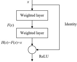
Residual network is composed of multiple serially connected residual blocks, specifically designed to facilitate deep feature learning while maintaining training stability. As illustrated in Fig. 1, each residual block mainly consists of two parallel functional subblocks. A shortcut connection links the input directly to the output feature map, effectively addressing the problems of gradient vanishing and network degradation that often occur during the training of deep networks. This architecture is particularly beneficial for bearing fault diagnosis, where accurate ex-traction of subtle fault features from complex vibration signals is crucial. The residual formulation introduces an auxiliary mapping:

where $x$ denotes the input of network, and let $H\left(x\right)$ be the desired underlying mapping. Then, the traditional training algorithm through fitting $H\left(x\right)$ is transformed equivalently to fitting the residual function $F\left(x\right)$:

when $F\left(x\right)$ reaches 0, $H\left(x\right)=x$. $H\left(x\right)=x$ represents the best solution mapping for a set of stacked network layers. If the network becomes deeper, it is hard for the model to directly fit the actual mapping $H\left(x\right)$. The residual structure starts to fit the residual mapping $F\left(x\right)$ by introducing shortcut connections, and the actual mapping $H\left(x\right)$ is expressed as $H\left(x\right)=F\left(x\right)+x$. When $F\left(x\right)=0$, an identity mapping $H\left(x\right)=x$ is obtained. The approximation of the actual mapping is achieved by minimizing the residual function $F\left(x\right)=H\left(x\right)-x$, which solves the performance degradation problem with network layer are stacked. So, compared with traditional training methods, it provides a more convenient and efficient approaches [20].

Fig. 1The structure of the residual block

2.2. Deep residual shrinkage network

To enhance robustness against noise, the deep residual shrinkage network (DRSN) was proposed as an extension of ResNet. DRSN integrates soft thresholding with channel-wise attention to selectively suppress noise-dominated features while preserving discriminative fault information. Specifically, within each residual shrinkage module, a subnetwork first estimates adaptive thresholds based on global feature statistics via a squeeze-and-excitation mechanism. These thresholds are then applied through a soft thresholding operator:

where $x$ and $y$ denote the input and output features, respectively, and $\tau >0$ is a learnable threshold. This design enables DRSN to effectively attenuate small-magnitude coefficients, while retaining salient fault-induced transients, which are easily masked in early-stage failures [20].

Despite its improved noise robustness, DRSN inherits the parameter-intensive nature of deep ResNet variants. The inclusion of additional attention subnetworks and multiple convolutional layers lead to a substantial increase in model complexity. In practical industrial applications, where computational resources and deployment costs are constrained, such high-parameter models are often impractical. Therefore, there remains a critical need for a lightweight yet robust fault diagnosis architecture that simultaneously achieves high accuracy under noisy conditions and maintains low computational overhead. This gap motivates our development of SE-SDCTNet, a compact model that synergistically combines sparse dense connectivity, adaptive soft thresholding, and channel attention to deliver both strong noise immunity and parameter efficiency.

3.1. Sparse dense compact thresholding block

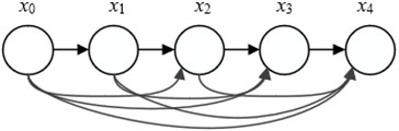
To enhance feature utilization efficiency and reduce the number of network parameters, we employ dense blocks. Unlike residual blocks, dense blocks promote the propagation of features and make more efficient use of features at different levels within each block. Each dense block is composed of multiple bottleneck layers that utilize dense connections between layers, maintaining consistent output sizes throughout the block. As shown in Fig. 2, this architecture ensures that the output of each layer contains the characteristic information from all preceding layers. In a dense connection setup, every layer receives feature maps from all previous layers as inputs and passes its own feature maps to all subsequent layers. This design not only increases the flow of information and gradients during training but also encourages feature reuse. The formula is as follows:

where $l$ corresponds to the input vector of the $l$-th layer; the operator $\oplus$ represents the concatenation operation of the feature vector; the function $H_l$ represents the nonlinear conversion function, which is a combination of Conv (1×1)-BN-ReLU. Here, BN refers to Batch Normalization, ReLU represents the activation function, Conv (1×1) indicates a convolution layer with a kernel size of 1×1, and Conv (3×3) indicates a convolution layer with a kernel size of 3×3. This mechanism ensures that each layer can directly access the final error signal, thereby improving the accuracy of the model in bearing fault diagnosis.

Fig. 2The structure of the dense block

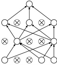
Inspired by sparse autoencoder [21], sparsity constraints are added to dense blocks to alleviate overfitting and suppress noise. By forcing the neural network to focus on the primary features of the data and ignore minor signals, this approach achieves stronger feature extraction and noise reduction capabilities. As illustrated in Fig. 3, the sparsity constraint ensures that only a portion of the neurons in the network are active. Through this sparse structure, key features in the data can be effectively extracted. It is implemented by L1 regularization.

Fig. 3The neural networks with sparsity constraints

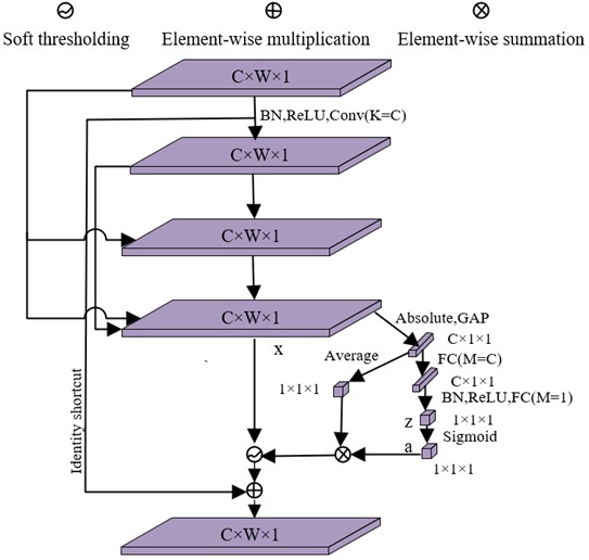
In this work, the SDCT block is proposed. As illustrated in Fig. 4, this module innovatively integrates a soft thresholding mechanism into a dense connection architecture, which is inspired by DRSN for capturing weak fault features in bearing vibration signals. Within the SDCT Block architecture, dense connections are implemented across all layers except the last: this design ensures full reuse of multilevel fault features from preceding layers, while feature concatenation is intentionally omitted at the final layer to reduce parameter complexity, addressing the industrial deployment barrier of large-parameter models. Additionally, sparse regularization is incorporated into the dense block to enforce sparsity constraints, further suppressing overfitting by limiting the activation of redundant neurons that may learn noise-related patterns, and guiding the network to focus on salient bearing fault features. The SDCT Block incorporates a dedicated subnetwork to estimate adaptive thresholds for soft thresholding, enabling targeted suppression of noise-related features in bearing vibration data. Specifically, Global Average Pooling (GAP) is first applied to the absolute values of the input feature map $x$ (which encodes spatial-frequency information of bearing vibrations), producing a one-dimensional channel-wise descriptor vector that aggregates global feature distribution across channels.

Fig. 4The structure of the sparse dense compact thresholding block

3.2. SE block

Sparsity ensures that certain channels within the SDCT blocks remain inactive, effectively preventing overfitting caused by redundant noise-related features in bearing vibration data. To further enhance the model’s ability to capture discriminative bearing fault features, multiple SDCT blocks are stacked together. However, in rolling bearing fault diagnosis scenarios. To address these issues, an SE block is introduced immediately after each SDCT block to dynamically amplify the weights of informative channels that encode key fault characteristics, while downplaying channels dominated by noise. The channel attention mechanism embedded in the SE block enables the model to identify and emphasize task-relevant features with only a marginal increase in model complexity and computational overhead. Implemented through the SE block as illustrated in Fig. 5, it comprises three sequential processes: Squeeze, Excitation, and Reweight.

Fig. 5The structure of the SE block

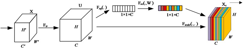
The globalization on feature map $F_{tr}$ is employed as the generalized function, and it yields feature map $G$, with a size of $W\times H\times C$, as the input of the attention mechanism:

where $F_{tr}$ represents the convolution operation, $U$ is the feature map, $H$ is the height, $W$ is the width, $C$ is the number of channels, and $D$ is the temporal depth. $v_c$ represents the $c$ -th convolution kernel, and $u_c$ represents the $c$ -th feature map. This process involves three distinct stages. Initially, the squeeze operation compresses features along the spatial dimension using global average pooling. Here, each spatial domain of size $H\times W$ is reduced to a single real number, which not only possesses a global receptive field but also aligns with the input feature’s channel count. These real numbers encapsulate the global distribution of responses across feature channels, enabling the network to gather global information even in early processing layers. The resulting output is a $1\times 1\times C$ vector, formulated as:

The next step is the Excitation operation, which is similar to the gate mechanism in a recurrent neural network. Each feature channel generates a corresponding weight based on the parameters $w$. These weights are obtained through learning, aiming to clearly model the correlation between feature channels. The operation can be expressed as:

where $w_1$ and $w_2$ denote fully-connected operations, $\delta$ is the ReLU function, and $\sigma$ is the sigmoid function. The last stage is the reweight stage, which regards the weight $s_c$ output by the Excitation stage as the importance of each feature channel after feature selection. Subsequently, these weights are weighted to the previous features $u_c$ channel by channel through multiplication operations, thereby recalibrating the original features in the channel dimension. The final output feature map can be expressed as:

Stacking SDCT blocks and SE blocks enhances the feature extraction capability of the bearing fault diagnosis model, making the network both lightweight and efficient while improving its noise resistance.

3.3. The proposed model

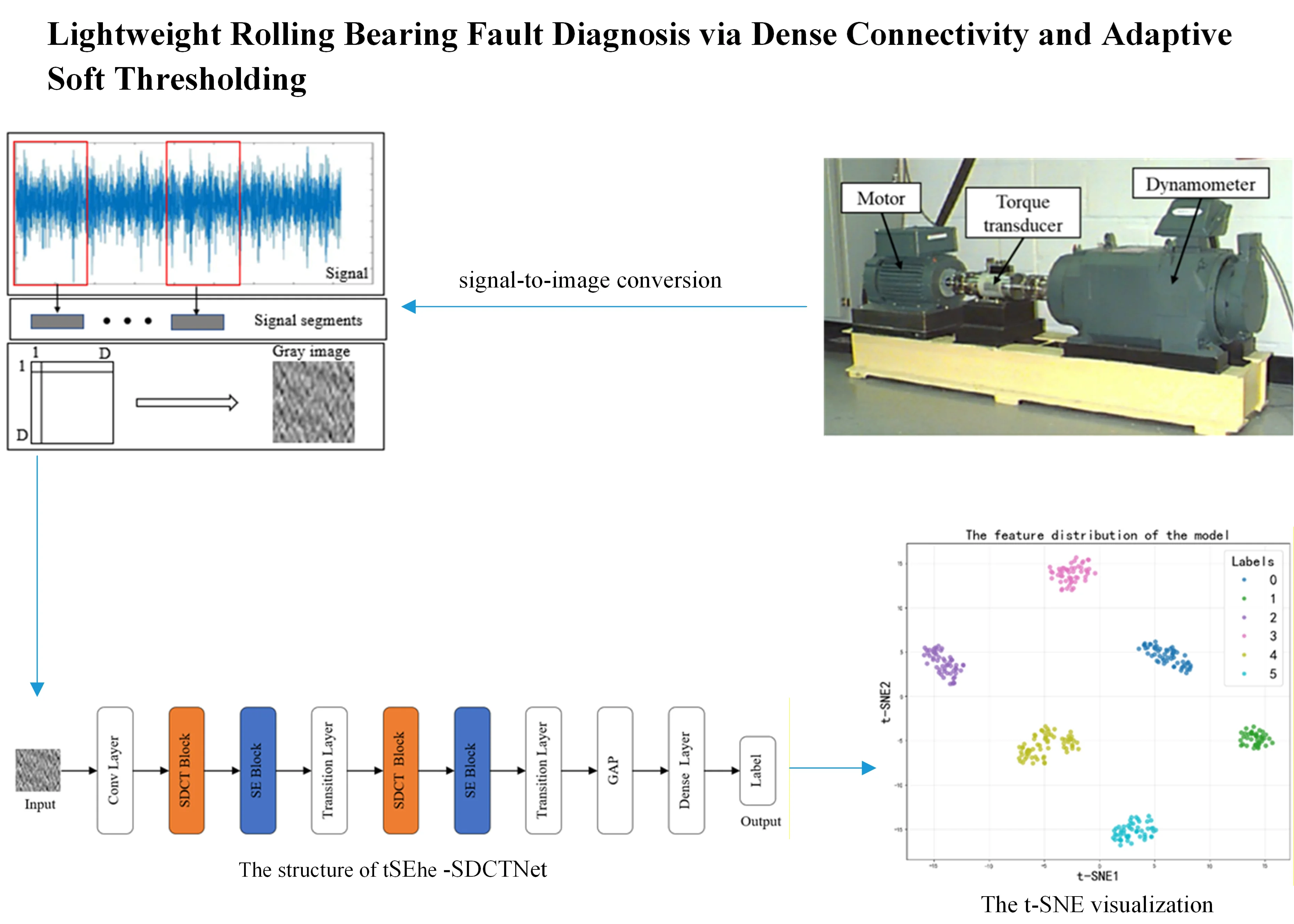
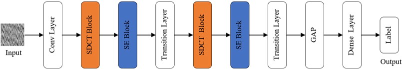
The fault diagnosis model proposed in this paper, named SE-SDCTNet, is composed of sequentially stacked Sparse-Dense Compact Thresholding (SDCT) blocks and Squeeze-and-Excitation (SE) blocks, with its overall architecture illustrated in Fig. 6. The model takes a 2D grayscale image (converted from 1D bearing vibration signals to preserve raw feature information) as input, and its structure follows a data-driven flow: standard convolution layers, a max-pooling layer, stacked SDCT blocks (each followed by a serial SE block), transition layers, a Global Average Pooling (GAP) layer, and Fully Connected (FC) layers.

The architecture begins with a standard 7×7 convolutional layer, processing the 32×32 input image to produce initial feature maps. To reduce parameter count and computational overhead, thereby accelerating training and inference, a 3×3 max‑pooling layer with stride 2 is applied immediately afterward. All subsequent convolutional layers use 3×3 kernels to balance feature extraction capability with computational efficiency. Following the initial pooling layer, two SDCT blocks are sequentially stacked, each followed by an SE block and a transition layer. The SDCT block employs a three‑layer convolutional structure (Fig. 4) to extract deep features: its dense connections enhance feature reuse by fully leveraging multi‑level fault‑related information from vibration signals, while its sparsity constraints suppress irrelevant noise and mitigate overfitting. The succeeding SE block adaptively recalibrates channel‑wise feature weights, emphasizing inter‑channel dependencies to further suppress noise and compensate for the channel‑independent nature of standard convolutions. Each transition layer then performs two key functions: first, a 1×1 convolution compresses the channel dimension to reduce model complexity and avoid feature redundancy; second, a max‑pooling layer with stride 2 downsamples the spatial size of the feature maps, enabling multi‑scale feature extraction in deeper layers. After processing through the stacked SDCT‑SE‑transition modules, the final feature map undergoes Global Average Pooling (GAP) to produce a one‑dimensional feature vector. This vector is mapped to output units corresponding to each fault category (including the normal state). For this multi‑classification task, a softmax activation is applied to generate class probabilities, and the category with the highest probability is selected as the final diagnostic label.

Fig. 6The structure of the proposed model

The module of multiscale feature extraction is built using dilated convolutions with diverse receptive fields [22]. This approach allows the network to capture information at different scales while preserving feature details. Dilated convolutions achieve a larger receptive field by introducing gaps into standard convolution kernels. These inserted holes are treated as zero-weight elements during the convolution operation on input feature maps. As a result, dilated convolutions can expand the receptive field without elevating computational expenses. By introducing the dilation rate $d$, the effective size of the convolution kernel in dilated convolutions is adjusted as follows:

where $k$ represents the size of the standard convolution kernel. In the SE-SDCTNet fault diagnosis model, different receptive fields are employed to acquire multi-scale feature information from vibration signals by configuring varying dilation rates for dilated convolutions. It is applied to a second SDCT block and d is set to 2.

3.4. Bearing image preparation from the vibration signal

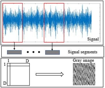
To leverage the powerful pattern recognition capabilities of CNNs which are inherently well-suited for processing two-dimensional data, one-dimensional vibration signals are converted into grayscale images. While time-frequency analysis is a common approach, it often relies on hand-crafted transformations that may discard valuable information or introduce complexity. Instead, we employ a direct and computationally efficient reshaping method, which provides the CNN with a structural view of the signal segment conducive to learning local temporal patterns [23].

Grayscale images of size $D\times D$ are generated by segmenting the raw vibration signal and reshaping the segment into a matrix. A length-$D^2$ segment – containing $D^2$ consecutive one-dimensional samples is first extracted; this length is selected so that the segment spans at least one complete revolution of the bearing. The samples are then arranged row-wise into a $D\times D$ matrix and normalized to the [0, 255] range, after which they are rounded to obtain integer pixel values. The resulting grayscale image is thus defined as:

where $L\left(h\right)$, $h=\text{ 1},\text{ 2}, \dots ,D^2$ represents the $h$-th the signal segment’s one-dimensional data point. $P\left(h,i\right)$ represents the value of the $h$-th row and the $i$-th column in the two-dimensional gray image with $h=\text{ 1},\text{ 2}, \dots ,D$, $i=\text{ 1},\text{ 2}, \dots ,D$. The minimal and maximal values of the intercepted signal are denoted by $\min (L)$ and $\max (L)$, respectively. $\text{Round}\left(.\right)$ is the rounding operator.

Fig. 7The process of signal-to-image conversion

3.5. Loss function formulation

Rolling bearing fault diagnosis is a multiclass classification problem. In the proposed SE-SDCTNet model, the softmax function is employed to estimate the probability distribution over fault classes. The softmax function transforms the raw output scores (logits) from the neurons into values within the range (0, 1), ensuring that their sum equals 1, thus forming a valid probability distribution. The model’s loss function is defined as the categorical cross-entropy between the predicted probability distribution and the true label distribution, which effectively measures the divergence between the model’s predictions and the ground truth, guiding the optimization process during training. It can be described as:

where $p\left(x\right)$ is the true distribution and $q\left(x\right)$ is the estimated distribution. $c$ is the number of categories. $y\left(i\right)$ is the true label and ${\widehat{y}}_i$ is predicted label of the model. In addition, L1 regularization is added to the loss function in the SDCT blocks. The final loss function is described as:

where $w_j$ is the weight parameter of the model, and $n$ is the total number of weight parameters, and $\lambda$ is the regularization strength coefficient, with a value of 0.001 in the proposed model. The model parameters undergo training by minimizing the loss function via the Adaptive Moment Estimation (Adam) optimization algorithm.

4.1. Experimental configuration

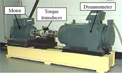
The CWRU dataset is extensively utilized as a benchmark for rolling bearing fault diagnosis [15]. Its data acquisition testbed is depicted in Fig. 8. In this setup, a faulty bearing was mounted on the test motor, and acceleration sensors at both the motor drive end and fan end recorded vibration data under varying loads. The dataset encompasses four types of bearing conditions: normal, inner race fault (IF), ball fault (BF), and outer race fault (OF).

Fig. 8The data acquisition testbed of the CWRU dataset

The experimental CWRU dataset comprised rolling bearing vibration signals under both normal and faulty conditions, with the data distribution summarized in Table 1. Specifically, six health states were examined at 1730, 1750, 1772, and 1797 RPM: normal state (label 0), inner race fault at 0.007 inches (label 1), inner race fault at 0.021 inches (label 2), ball fault at 0.021 inches (label 3), outer race fault at 0.007 inches (label 4), and outer race fault at 0.021 inches (label 5). Each sample contained 1024 sampling points. The input image samples for the SE-SDCTNet model were created through signal-to-image conversion, yielding 32×32 images. A total of 2400 samples were utilized, with 300 training samples and 100 test samples for each type.

4.2. Ablation experiments on the CWRU dataset

To validate the effectiveness of each key component in the proposed SE-SDCTNet architecture, we conduct a comprehensive ablation study on the CWRU dataset under the four operating conditions (1730, 1750, 1772, and 1797 RPM). All variants share identical data splits, training procedures, and evaluation protocols. Specifically, models are optimized using the Adam optimizer with an initial learning rate of 0.0001. A learning rate decay strategy is applied, where the learning rate is multiplied by a factor of 0.96 every 5 epochs.

The ablation experiment results of SE-SDCTNet on the CWRU dataset (tested in noise-free environments) are presented in Fig. 9: under these ideal conditions, all models (DenseNet, SE-DenseNet, SDCTNet, and SE-SDCTNet) achieve 100 % diagnostic accuracy, reflecting strong fault classification performance across architectures. The mechanism behind this consistent high performance can be visualized via the t-distributed stochastic neighbor embedding (t-SNE) results of SE-SDCTNet under four operating conditions (1730/1750/1772/1797 RPM) in Fig. 10. In these plots, samples of different fault categories form distinct, non-overlapping clusters, this clear feature separation directly reflects SE-SDCTNet’s ability to capture unique fault characteristic patterns, which underpins the 100 % accuracy observed in Fig. 9. This alignment between high accuracy and well-separated feature clusters stems from ideal noise-free environments: bearing vibration signals carry unobscured fault-related spectral information, allowing both SE-SDCTNet and other baseline models to easily distinguish distinct fault patterns.

Fig. 9Ablation experiment results of SE-SDCTNet on the CWRU dataset

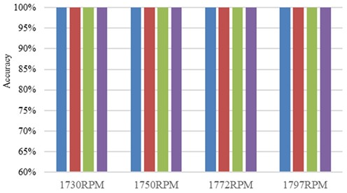
Fig. 10The t-SNE visualization of the SE-SDCTNet under four operating conditions

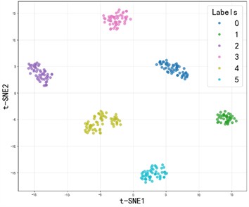
a) 1730RPM

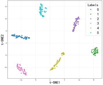
b) 1750RPM

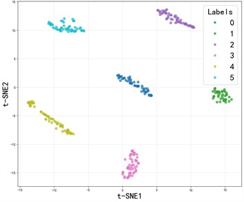
c) 1772RPM

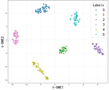
d) 1797RPM

However, real industrial scenarios involve significant background noise, which obscures fault features and degrades feature discriminability. To simulate this practical challenge, Gaussian noise was introduced into the test set’s vibration signals, with signal-to-noise ratio (SNR) quantifying noise intensity, this framework will enable systematic evaluation of whether SE-SDCTNet can maintain clustered, separable features (and high accuracy) under varying noise levels. The SNR was employed to quantify noise intensity, enabling a systematic assessment of each model’s robustness and its ability to preserve feature discriminability under varying levels of noise interference. The SNR is defined as [26]:

where $P_{signal}$ and $P_{noise}$ denote the signal and noise powers, respectively.

Fig. 11Ablation experiment results of SE-SDCTNet with noise interference at 1797 RPM

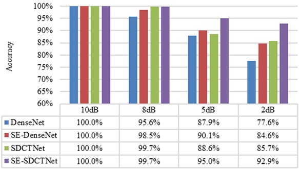
Fig. 11 illustrates the diagnostic accuracy of various model variants under different noise levels (from 10 dB to 2 dB) when classifying six types of bearing faults, with 100 test samples per category. The results demonstrate a clear degradation in performance as noise intensity increases for all models. Specifically, DenseNet achieves high accuracy (100 %) under low-noise conditions but drops sharply to 77.6 % under 2 dB noise – a decline of 22.4 percentage points, indicating limited robustness in noisy environments. Incorporating SE blocks into DenseNet (SE-DenseNet) improves noise robustness, maintaining 84.6 % accuracy at 2 dB noise, representing only a 15.4 percentage point drop. This improvement arises from the SE module’s ability to adaptively recalibrate channel-wise feature responses, enhancing the representation of fault-relevant information while suppressing irrelevant activations. Replacing conventional dense blocks with SDCT blocks (SDCTNet) further enhances performance, achieving 85.7 % accuracy under 2 dB noise (a 14.3 percentage point drop), demonstrating the effectiveness of sparsity constraints in reducing redundant neuron activation and filtering out noise interference. When both SE and SDCT blocks are combined in the proposed SE-SDCTNet, the model achieves the highest overall accuracy across all noise levels. Notably, it maintains 92.9 % accuracy even under severe 2 dB noise, with only a 7.1 percentage point reduction from the noise-free case. This superior robustness stems from the synergistic interaction between the two mechanisms: the SDCT block enforces sparse representations to suppress noise, while the SE block selectively amplifies salient features through channel attention. Together, they enable SE-SDCTNet to achieve an optimal balance between lightweight design and strong noise resilience, significantly outperforming individual components and baseline architectures.

4.3. Comparison of different diagnostic models on the CWRU dataset

For comparison, seven well-established deep learning baselines including LeNet5 [24], LiNet [19], Swin Transformer [25], ResNet18 [26], SENet18 [16], DenseNet [27], and MobileNetV2 [18] were also adopted for bearing fault diagnosis on the CWRU dataset. These networks span both classical CNNs and modern architectures about attention for bearing fault diagnosis. LeNet5 is one of the earliest and most representative lightweight convolutional networks. It employs 5×5 convolutions followed by 2×2 max-pooling. LiNet is a specialized lightweight network explicitly tailored for mechanical fault diagnosis. It is realized by one convolutional block with 3×1 convolution kernels, two light modules consisting of uneven-sized convolution blocks, residual structures, and one convolutional block with 1×1 convolution kernels. The Swin Transformer splits input images into patches for embedding, processes them via 4 Swin Transformer blocks, then outputs classifications through layer norm, global pooling, and a dense layer. The ResNet18 contains one 3×3 convolutional stem, eight basic residual blocks, GAP, and an FC classifier. The SENet18 augments ResNet18 by inserting SE blocks into every residual block. The DenseNet comprises an initial 3×3 convolution, 58 densely connected blocks, three transition layers, GAP, and an FC layer. MobileNetV2 is a highly efficient, lightweight convolutional architecture built upon inverted residuals and linear bottlenecks. Unlike MobileNetV1, which uses depthwise separable convolutions throughout, MobileNetV2 introduces an expansion layer before the depthwise convolution to increase representational capacity, followed by a linear projection layer that preserves information flow in the low-dimensional space.

All subsequent experiments used identical data splits, training schedules, and evaluation protocols. The models tested include LeNet5, LiNet, Swin Transformer, ResNet18, SENet18, DenseNet, and MobileNetV2. These models were trained using the Adam optimizer. Decay steps refer to the number of iterations after one decay and decay rate refers to the learning rate after one decay. Parameters refers to the number of model parameters, in millions.

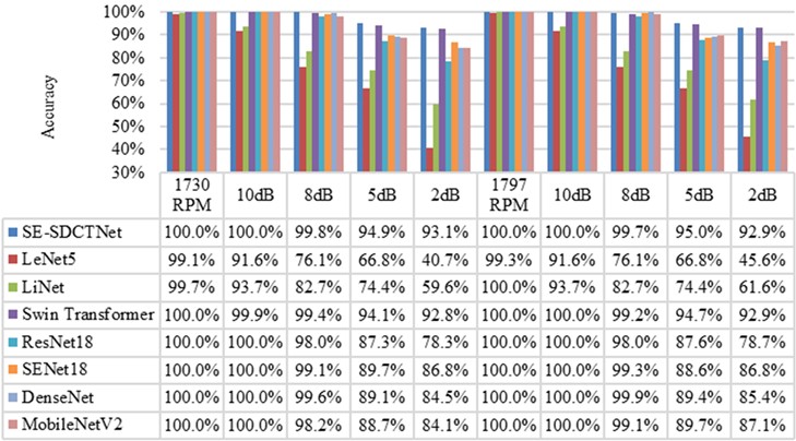
Fig. 12 compares the diagnostic accuracy of multiple models, including the proposed SE-SDCTNet, across a range of noise intensities (from noise-free to 2 dB) on six rolling bearing fault types, with 100 test samples per category. At 1730 RPM, basic lightweight models such as LeNet5 and LiNet achieve high accuracy (99.1 % and 99.7 %, respectively) under noise-free conditions, confirming their effectiveness in ideal, low-interference scenarios. However, their performance degrades sharply as noise increases: under the harsh 2 dB condition, LeNet5’s accuracy drops sharply to 40.7 % (a decline of 58.4 percentage points), and LiNet falls to 59.6 % (a 40.1-point reduction). This severe sensitivity to noise renders them unsuitable for real industrial environments, where noise is inevitable. Mainstream models with higher parameter counts, such as ResNet18, SENet18, and DenseNet, exhibit stronger noise robustness. For instance, ResNet18 maintains 78.3 % accuracy under 2 dB noise. Nevertheless, their considerable model complexity hinders deployment on resource-constrained edge devices, a key practical requirement for industrial bearing diagnosis. In contrast, SE-SDCTNet achieves 100 % accuracy in both noise-free and 10 dB noise at 1730 RPM, and retains 93.1% under severe 2 dB noise – a decrease of only 6.9 percentage points. This trend is consistent at 1797 RPM, where SE-SDCTNet maintains leading accuracy across all noise levels, outperforming both lightweight and large-parameter counterparts. This robustness stems from the synergistic design of SE-SDCTNet’s core components: the SDCT block suppresses noise through sparsity constraints, limiting activation of redundant neurons; the SE block adaptively recalibrates channel-wise feature responses, preserving critical fault signatures even when sparse filtering removes less relevant channels; and dilated convolutions expand the receptive field without added computation, retaining global fault characteristics. Together, these mechanisms allow SE-SDCTNet to achieve an optimal balance – surpassing conventional lightweight models in noisy settings through superior robustness, while exceeding large-parameter networks in deployment efficiency due to its compact architecture.

Fig. 12Composed experiment results of SE-SDCTNet on the CWRU dataset

To further analyze the experimental results, additional evaluation metrics (precision, recall, and F1-score) were used. Table 3 presents the precision, recall, and F1-score of the SE-SDCTNet model when subjected to a noise level of 2 dB. These metrics serve to assess the overall diagnostic performance of the SE-SDCTNet model in the presence of noise interference and are defined as follows:

where TP denotes the count of positive samples accurately predicted as positive; FP represents the number of negative samples mistakenly predicted as positive; FN signifies the positive samples incorrectly predicted as negative; and TN indicates the negative samples correctly predicted as negative. Additionally, P, R, and F stand for precision, recall, and the F1-score, respectively.

The classification results indicate that the model performs well overall in identifying various samples, with the Precision, Recall, and F1-score for different fault types and the normal state all remaining above 0.87. Among them, the fault type BF007 corresponding to label 1 achieves the optimal recognition performance, with Precision, Recall, and F1-score all reaching 1.00, realizing perfect classification. The fault types IF021 (label 2) and BF021 (label 3) also perform excellently, with F1-scores of 0.97 and 0.94 respectively, demonstrating that the model has high accuracy and completeness in identifying these two types of faults. In comparison, the OF007 (label 4) and normal state (label 0) show slightly weaker performance, with F1-scores of 0.88 and 0.89 respectively, but they are still at a good level. Overall, the model can effectively distinguish between different fault types and the normal state.

Fig. 13The confusion matrices of the SE-SDCTNet in 8dB and 2dB

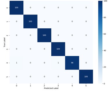
a) 8 dB

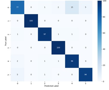
b) 2 dB

To further visualize the fine-grained classification performance of SE-SDCTNet at 1730 RPM, the confusion matrices of SE-SDCTNet under 8 dB and 2 dB noise conditions are presented in Fig. 13, with fault labels corresponding to the definitions in Table 1 (0: Normal, 1: IF007, 2: IF021, 3: BF021, 4: OF007, 5: OF021). At 8 dB SNR (Fig. 13(a)), the model achieves near-perfect classification with an overall accuracy of 99.7 %. Most fault types (e.g., IF007, BF021, OF007, OF021) are correctly identified across all 100 samples. The only errors are two OF007 (Label 4) samples misclassified (one as Normal and one as BF021), demonstrating the model’s strong discriminative power in moderate-noise environments. Under the harsher 2 dB condition (Fig. 13(b)), the model maintains a high overall accuracy. Misclassifications are primarily concentrated between specific pairs: 15 Normal samples are misclassified as OF007, 5 OF021 sample is confused with Normal, and 3 IF021 samples are scattered among Normal, BF021, and OF007. This error pattern aligns with the inherent subtlety of the corresponding fault signatures. Normal samples, lacking fault-specific components, are prone to being mislabeled as low-amplitude faults (e.g., BF021) under high noise. Similarly, OF021 features are weaker than those of larger-magnitude faults, leading to confusion with the Normal state. Notably, the confusion matrix retains strong diagonal dominance, with 100 % correct identification for faults like IF007 and BF021. This indicates that SE-SDCTNet possesses reliable fault discrimination capability even in challenging noise conditions.