Application of GSABO-VMD-KELM in rolling bearing fault diagnosis

1. Introduction

The health condition of rolling bearings is directly related to the safe and stable operation of equipment. Timely detection of faults in key rolling bearings is crucial for ensuring the reliability and safety of machinery [1-3]. Once a rolling bearing in mechanical equipment fails, it may lead to equipment downtime, production interruptions, or even safety accidents, which can have a severe impact on production and operations [4-6]. Therefore, it is especially important to diagnose and predict bearing faults in a timely manner. However, due to the complex working environment of mechanical equipment, bearings are susceptible to issues such as wear and fatigue [7], which increases the difficulty of fault diagnosis. Therefore, researching high-precision bearing fault diagnosis methods is of great significance for enhancing the safety and reliability of mechanical equipment.

The fault signals of rolling bearings exhibit non-stationary and nonlinear characteristics [8]. Therefore, signal decomposition algorithms are regarded as useful tools for extracting fault features [9]. Empirical Mode Decomposition (EMD) [10] decomposes signals based on the time-scale characteristics of the data itself, without the need to preset any basis functions. Once proposed, this methodology has been extensively and successfully implemented in the domain of fault diagnosis. Nevertheless, the ultimate efficacy and the mode admixture have significantly constrained its applicability. To effectively resolve these challenges, a sequence of recursive decomposition methodologies has been systematically developed, such as Local Mean Decomposition (LMD) [11], and Ensemble Empirical Mode Decomposition (EEMD) [12], Improved Complete Ensemble Empirical Mode Decomposition with Adaptive Noise (ICEEMDAN) [13]. Nevertheless, the recursive decomposition approach fails to fundamentally resolve the issue of mode mixing [14]. In addressing this particular concern, Konstantin et al. [15] proposed the Variational Mode Decomposition (VMD) technique. Due to its superior filtering capabilities and rigorous theoretical foundation, VMD has gained widespread popularity and recognition among researchers since its introduction [16]. Meng [17] proposed an enhanced VMD method that precisely extracts fault features through adaptive adjustment of the penalty factor. Yang et al. [18] employed the simulated annealing (SA) algorithm to optimize VMD parameters, successfully achieving early fault detection. Wang et al. [19] introduced a particle swarm optimization-based VMD method for complex rotating machinery fault diagnosis. Although these optimization algorithms demonstrate satisfactory performance in parameter optimization, these algorithms frequently converge to local optima, potentially leading to overfitting or underfitting scenarios that may degrade overall performance.

Following the completion of feature extraction from rolling bearing fault signals, the extracted feature matrix requires identification and diagnosis. With the rapid development of science and technology, deep learning diagnostic models are increasingly applied in the fault diagnosis of rolling bearings. Such as dynamic collaborative adversarial domain adaptation networks (DCADAN) [20], task-oriented Theil index-based meta-learning networks (TTIMN-GCS) [21], attention-guided hierarchical wavelet convolutional networks (AHWCN) [22]. Although these methods have all demonstrated excellent performance in the application of fault diagnosis for rolling bearings, they still face problems such as complex computation, long diagnosis time, lack of hyperparameter optimization strategies, and reliance on prior knowledge of fault features for parameter setting. Common fault recognition models include Backpropagation Neural Networks (BPNN) [23] and Extreme Learning Machines (ELM) [24], among others. The BP neural network fault identification model suffers from several limitations, including high learning costs and susceptibility to overfitting when handling noisy data [25]. Meanwhile, ELM faces challenges such as random initialization of input weights and potential overfitting issues [26]. In response to the issues, Huang et al. [27] proposed the KELM algorithm, which combines the kernel method with the framework of extreme learning machines. It can effectively handle nonlinear relationships and high-dimensional data, offering fast training speeds and strong generalization capabilities. However, the KELM algorithm also has some limitations, as its performance is significantly influenced by the regularization coefficient $C$ and the kernel function parameter$g$. If $C$ and $g$ are not selected properly, they may negatively impact the model’s classification accuracy. Zhao et al. [28] employed the Particle Swarm Optimization (PSO) algorithm to optimize the regularization coefficient $C$ and kernel function parameter $g$ of the KELM algorithm, thereby enhancing its effectiveness in gearbox fault diagnosis. Yang et al. [29] proposed a rolling bearing fault diagnosis method based on variational mode decomposition optimized by an improved artificial fish swarm algorithm and multi-feature vector fusion with extreme learning machines. However, both particle swarm optimization and artificial fish swarm algorithms are prone to premature convergence and getting trapped in local optima, exhibiting poor robustness. The subtraction-average-based optimization algorithm is a novel optimization algorithm [30] with outstanding optimization performance. Lu Fan [31] verified that using the subtraction-average-based optimizer (SABO) to optimize the selection process of the mode number and penalty factor in variational mode decomposition (VMD) improved the classification accuracy of rolling bearing fault diagnosis. However, the SABO algorithm also has the issue of easily falling into local optima. In their study on rolling bearing fault diagnosis based on adaptive local iterative filtering (ALIF) and time-shifted multi-scale fluctuation dispersion entropy (TMFDE), Zhao Jiahao et al. [32] noted that the MFDE method achieved a maximum classification accuracy of 82 % and a minimum classification accuracy of 74 %, with a difference of 8 %. This indicates that falling into local optima significantly impacts the classification accuracy of rolling bearing fault diagnosis.

In summary, to further improve the classification accuracy of rolling bearing fault diagnosis, this paper proposes an improved subtraction-average-based optimizer algorithm, GSABO. The method combines GSABO with VMD and KELM, where the GSABO-KELM model classifies the feature matrix formed by calculating the envelope entropy of the IMF components screened after GSABO-VMD decomposition. Ultimately, this approach identifies the fault types of rolling bearings. The superiority of the proposed method is validated using datasets from Case Western Reserve University and Xi’an Jiaotong University.

The main contributions of this paper are as follows:

(1) The SABO algorithm is improved by incorporating chaotic mapping strategies and the golden sine algorithm. Compared with other optimization algorithms, the proposed GSABO algorithm demonstrates superior performance in optimization accuracy, computational efficiency, and convergence capability.

(2) The GSABO algorithm is employed to achieve adaptive selection of VMD parameters, thereby reducing the complexity of the problem.

(3) By integrating the GSABO algorithm with VMD and KELM, this study provides enhanced accuracy and convergence for rolling bearing mechanical fault diagnosis, offering new possibilities for existing fault diagnosis technologies.

2. Fundamental theory

2.5. Fault diagnosis process

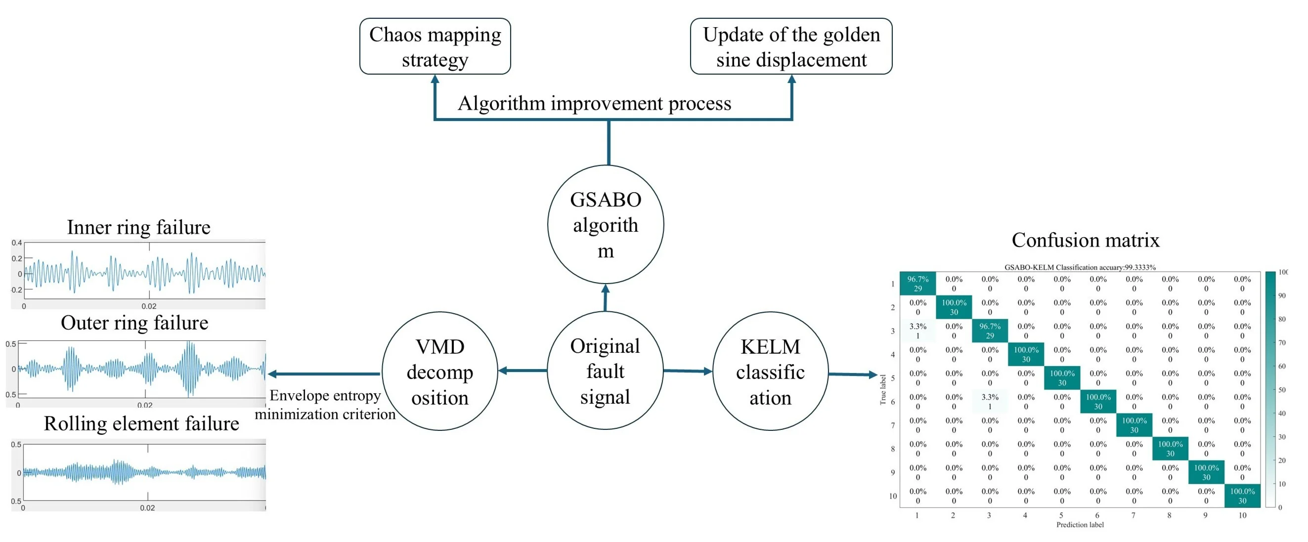
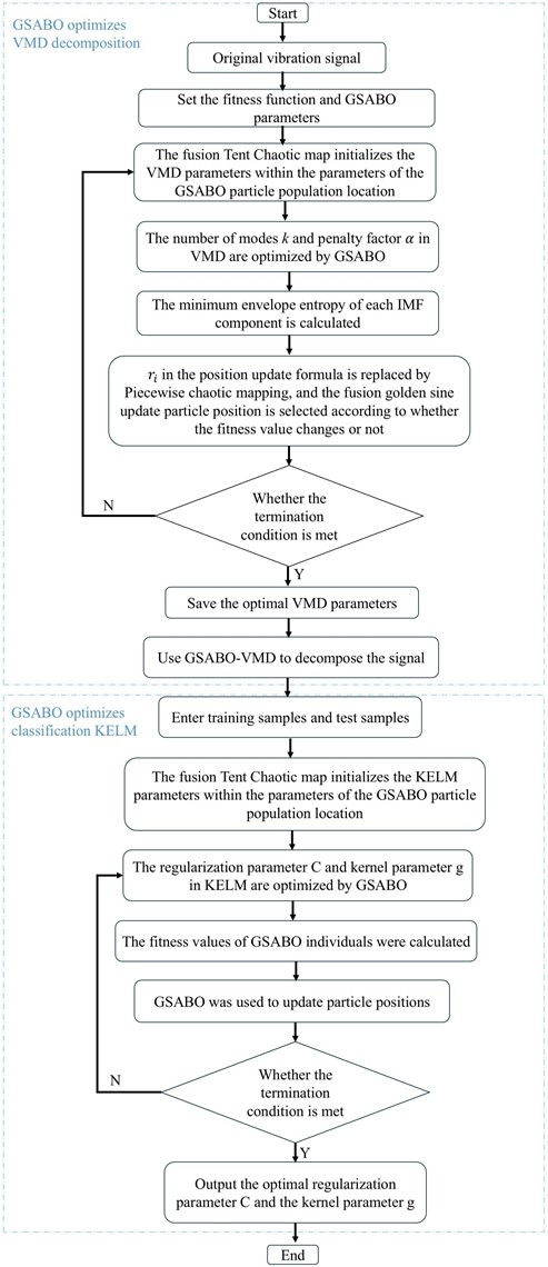
The overall flowchart for fault diagnosis is shown in Fig. 1. The specific steps for optimizing VMD and KELM using GSABO are as follows:

Step 1: Input the original vibration data and set the fitness function as well as the GSABO parameters.

Step 2: Initialize the population and positions of particles in the GSABO algorithm for VMD parameters using the Tent chaotic map.

Step 3: Decompose the signal using VMD and calculate the envelope entropy of each IMF component

Step 4: Replace $r_i$ in the position update formula with the Piecewise chaotic map and selectively fuse the golden sine strategy to update particle positions based on fitness value variations.

Step 5: Evaluate whether to update the current best solution. If the fitness value of the particle's current position is better than the historical best fitness value, update this position as the new position for the corresponding population particle and save this fitness value as the optimal fitness value

Step 6: Perform iterative cycles until the preset stopping criteria are met.

Step 7: Decompose the signal using the optimal parameters obtained from GSABO-optimized VMD.

Step 8: Divide the dataset into training samples and testing samples.

Step 9: Initialize the population and positions of GSABO particles within the KELM parameter range by incorporating the Tent chaotic mapping.

Step 10: Optimize the regularization coefficient $C$ and kernel parameter $g$ in KELM using GSABO, and calculate the fitness value of each GSABO individual

Step 11: Update particle positions using the GSABO algorithm.

Step 12: Determine whether the termination criteria are met. If satisfied, proceed to the next step; otherwise, return to Step 10.

Step 13: Obtain the optimal regularization parameter and kernel parameter.

Fig. 1Flowchart of the GSABO-VMD-KELM fault diagnosis method

3. Simulation experiment

To demonstrate the advantages of the improved SABO optimization algorithm incorporating golden sine (GSABO) over SABO and other traditional optimization algorithms, the F1, F5, and F8 functions from the CEC2005 benchmark test set were selected for testing and comparison. The expressions of these functions are shown in Table 1, and the comparison results are illustrated in Fig. 2-4.

Fig. 2Comparison of optimization results on F1 function

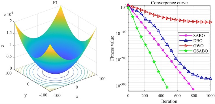
Fig. 3Comparison of optimization results on F5 function

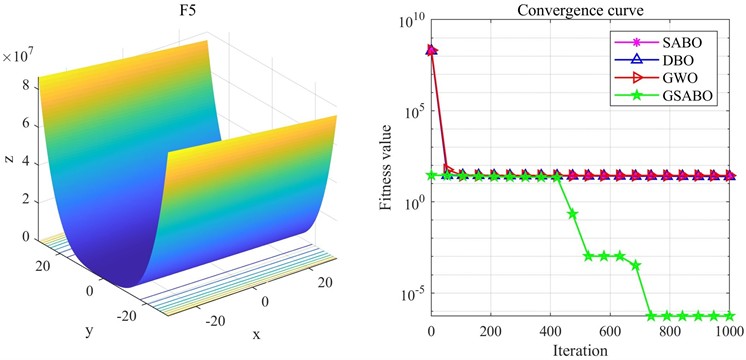
Fig. 4Comparison of optimization results on F8 function

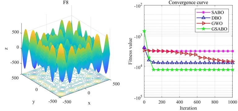
From the comparative results, it can be observed that F5 and F8 are among the most challenging functions in the CEC2005 benchmark set for evaluating optimization algorithm performance. For F5, whose theoretical minimum is 0, the improved algorithm achieved an optimization value of 6.19×10^-6, whereas the Whale Optimization Algorithm (WOA), Dung Beetle Optimizer (DBO), and Subtraction-Average-Based Optimizer (SABO) all yielded values around 27. For F8, a multimodal function with multiple peaks, intelligent algorithms are highly prone to falling into local optima during optimization. Its theoretical minimum is –12569.5, and GSABO obtained a near-optimal value of –12569.4737, which is extremely close to the theoretical optimum. Combined with the results in Fig. 4, GSABO outperforms the other three algorithms and exhibits faster convergence speed. In summary, based on the test results of three functions, the improved GSABO demonstrates significant advantages in both convergence speed and final optimization accuracy compared to the other algorithms.

4. Experimental analysis

4.1. Case 1

4.1.1. Data collection

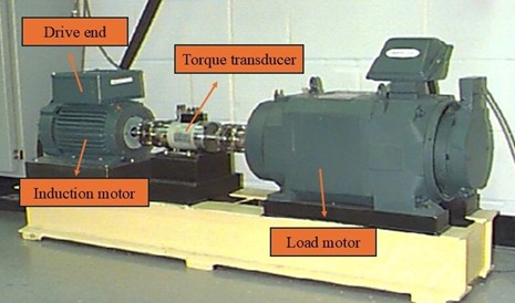
To validate the effectiveness of the GSABO algorithm in rolling bearing fault diagnosis, an empirical evaluation was conducted using the bearing dataset from CWRU. Fig. 5 shows the basic configuration of the test rig. The specifications of the bearing data are as follows: SKF bearings were used, the motor was running at a speed of 1797 r/min, and the load was set to zero horsepower, with a sampling frequency of 12 kHz. The dataset covers four different fault conditions: normal state, inner race fault, outer race fault, and ball fault, with corresponding fault diameters of 0.007 inches, 0.014 inches, and 0.021 inches, respectively.

There are 10 types of faults. For the convenience of the experiment, these faults are coded as follows: “1” represents the normal state, “2-4” represent inner ring faults with diameters of 0.007, 0.014, and 0.021 inches, “5-7” represent rolling element faults with diameters of 0.007, 0.014, and 0.021 inches, and “8-10” represent outer ring faults with diameters of 0.007, 0.014, and 0.021 inches. Each fault signal contains 2048 sampling points, and there are 120 fault samples collected for each type of fault, with 90 samples used for the training set and 30 samples used for the testing set.

Fig. 5Bearing data acquisition platform of Case Western Reserve University

4.1.2. Fault signal GSABO-VMD decomposition

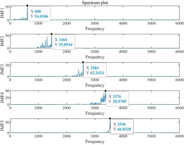
After acquiring the fault signal, the first step is to set the parameters for GSABO-VMD. The population size of GSABO is set to 15, and the maximum number of iterations is set to 20. The decomposition layer $k$ and the penalty factor $\alpha$ are optimized within the ranges $k\in \left[\mathrm{3,10}\right]$ and $\alpha \in \left[\mathrm{100,2500}\right]$, with the objective of minimizing the envelope entropy. Taking a fault signal with a fault size of 0.007 inches as an example, the optimization results obtained through GSABO are $\left(k,\alpha \right)=\left(\mathrm{5,482}\right)$. The VMD decomposition results optimized by GSABO are shown in Fig. 6, while the decomposition results using the default parameter set [4, 2000] [35] are shown in Fig. 7.

Fig. 6VMD frequency spectrum decomposition diagram after parameter optimization

According to the theoretical frequency calculation formula of the inner ring fault of rolling bearings, as shown in Eq. (22):

22

$f_i=0.5zf\left(1+\frac{d}{D}\cos \alpha \right),$

where, $d$ represents the diameter of the rolling element; $D$ represents the raceway pitch diameter; $\alpha$ represents the contact angle of the bearing; $z$ represents the number of rolling elements; $f$ represents the frequency conversion.

Fig. 7VMD frequency spectrum decomposition diagram with default parameters

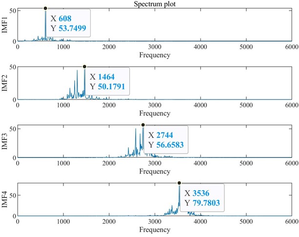
The theoretical frequency of the inner ring fault of the 6205-2RS bearing can be calculated as 134.775 Hz, the fault frequency of the IMF4 component in Fig. 6 is 3376 Hz, which is very close to the 25 times fault frequency of the inner ring at 3369.375 Hz, while the fault frequency decomposed in Fig. 7 differs significantly from the fault frequency of the inner ring.

The optimized VMD decomposition includes inner ring failure frequency. As observed from the amplitude of the spectrogram, this component represents significant features of the original signal that were overlooked under default parameters. The results demonstrate that the optimized parameters can more effectively characterize the features of the original signal.

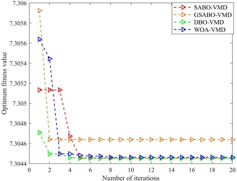
Fig. 8 shows the evolutionary curve comparison of the algorithms. GSABO achieves convergence at the 3rd generation, while the unimproved SABO converges at the 6th generation. DBO completes convergence at the 6th generation, and WOA reaches convergence at the 8th generation. Notably, GSABO demonstrates significantly better optimization performance than the other three algorithms, which clearly illustrates the superiority of the proposed optimization method.

4.1.3. Feature extraction from signal decomposition results

Prior to feature extraction from the IMF components obtained through GSABO-VMD decomposition, it should be noted that a smaller envelope entropy value indicates richer fault information, while a larger value suggests less fault information [36]. Given that each IMF component contains different characteristic quantities, we select the IMF component with the smallest envelope entropy for feature extraction. The calculated envelope entropy values for each IMF component are presented in Table 2.

Table 2Computed envelope entropy values

IMF1	IMF2	IMF3	IMF4	IMF5
7.3045	7.30464	7.30471	7.30445	7.30451

Among these five IMF components, IMF4 has the smallest envelope entropy value, so it is selected as the optimal IMF component. After completing the IMF component selection, we calculate time-frequency domain features including mean and variance of the optimal IMF components as characteristic indicators for feature extraction.

Fig. 8Performance comparison of convergence curves

Using the same methodology as presented in the provided examples, the parameter combinations $\left(k,\alpha \right)$ for these 10 fault types and their corresponding optimal IMF components can be obtained. Detailed data are shown in Table 3.

Table 3Optimal VMD parameters and corresponding IMF components

Condition	Fault Size	Label	$\left(k,\alpha \right)$	Optimal IMF
Normal	0.007	1	(8, 1369)	IMF8
IRF	0.007	2	(5,482)	IMF4
IRF	0.014	3	(7, 3000)	IMF5
IRF	0.021	4	(3, 190)	IMF3
REF	0.007	5	(6, 583)	IMF3
REF	0.014	6	(4, 3000)	IMF3
REF	0.021	7	(8, 158)	IMF5
ORF	0.007	8	(6, 705)	IMF6
ORF	0.014	9	(8, 152)	IMF3
ORF	0.021	10	(4, 1274)	IMF4

4.1.4. Fault feature identification

By computing time-frequency domain features of the screened IMF components as characteristic indicators, a fault feature vector matrix is constructed for fault type classification using GSABO-KELM. The samples are fed into KELM, with its kernel parameter $C$ and regularization coefficient $g$ optimized by GSABO. For the algorithm parameters, the population size is set to 20, the maximum iterations to 30, and the optimization ranges for $C$ and $g$ are set as [0, 1000] respectively. The optimization process uses classification accuracy as the fitness function. The best parameter set $\left(C,g\right)=\left(\mathrm{1000,0.546}\right)$ obtained through GSABO-KELM optimization yields an accuracy of 99.3333 %, while Fig. 9 shows the test set confusion matrix using GSABO-VMD decomposition.

Fig. 9Confusion matrix of GSABO on the test set

Fig. 10Confusion matrix of SABO on the test set

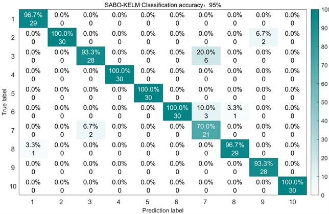
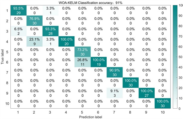
For comparative analysis, we employed the previously benchmarked unoptimized SABO, DBO, and WOA algorithms for VMD decomposition of the experimental dataset. Maintaining identical feature extraction and classification procedures, the test set recognition accuracies achieved were 95 %, 93.6667 %, and 91 % respectively. The corresponding test results and confusion matrices are presented in Fig. 10 through 12.

Following the procedure, the GSABO-VMD-KELM algorithm was compared with existing state-of-the-art methods, introduce accuracy, precision, recall, and F1 score as evaluation metrics, the formula is as follows:

23

$Accuary=\frac{TP+TN}{TP+FP+TN+FN},$

24

$Precision=\frac{TP}{TP+FP},$

25

$Recall=\frac{TP}{TP+FN},$

26

$F1=2\times \frac{Precision\times Recall}{Precision+Recall},$

where, True Positive (TP): the model predicted a positive case and it was a positive case; False Positive (FP): the model predicted a positive case, but it was a negative case. True Negative (TN): the model predicted a negative case, and it was a negative case. False Negative (FN): the model predicted a negative case, but it was a positive case.

Fig. 11Confusion matrix of DBO on the test set

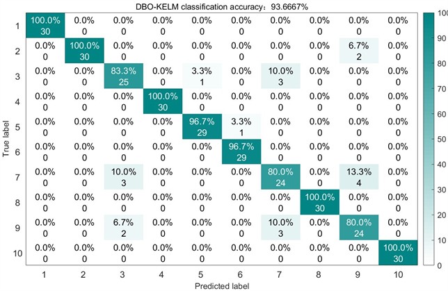
Fig. 12Confusion matrix of WOA on the test set

The preparation rates of different fault diagnosis models are shown in Table 4, the precision is presented in Table 5, recall rates are presented in Table 6 and the F1 scores are illustrated in Table 7.

In the comprehensive assessment, both GSABO-VMD-KELM and SABO-VMD-KELM exhibited outstanding performance across the four diagnostic metrics. Nevertheless, SABO-VMD-KELM displayed relatively lower accuracy and F1 score in diagnosing the seventh category of faults, indicating a minor limitation. Conversely, Method 1 effectively mitigated the issue of misdiagnosis, demonstrating robust diagnostic capabilities.

Table 4Performance comparison of different algorithms

Number	Algorithm Name	Classification accuracy
1	GSABO-VMD-KELM	99.3333 %
2	SABO-VMD-KELM [37]	95 %
3	DBO-VMD-KELM [38]	93.6667 %
4	WOA-VMD-KELM [39]	91 %
5	VMD-ELM [40]	83.3333 %
6	VMD-KELM [41]	89.6667 %
7	VMD-CNN [42]	87.6667 %
8	DCADAN [20]	90 %
9	TTIMN-GCS [21]	92.3333 %
10	AHWCN [22]	93 %

Table 5Comparative analysis of (Precision %) across various methodologies

Algorithm Name	Fault labels
	1	2	3	4	5	6	7	8	9	10
GSABO-VMD-KELM	96.7	100	96.7	100	100	100	100	100	100	100
SABO-VMD-KELM [37]	96.7	100	93.3	100	100	100	70.0	96.7	93.3	100
DBO-VMD-KELM [38]	100	100	83.3	100	96.7	96.7	80	100	80	100
WOA-VMD-KELM [39]	93.5	76.9	93.3	100	73.2	100	90.9	100	100	100
VMD-ELM [40]	100	100	86.7	100	60	30	83.3	100	73.3	100
VMD-KELM [41]	70	96.8	85.3	100	93.8	95.2	78.9	85.3	96.6	100
VMD-CNN [42]	62.5	100	77.1	100	100	100	86.2	88.2	87.5	100
DCADAN [20]	100	100	86.7	100	96.7	53.3	96.7	100	66.7	100
TTIMN-GCS [21]	100	100	86.7	100	100	80.0	90.0	100	66.7	100
AHWCN [22]	82.4	93.8	83.3	100	93.8	93.1	92.0	96.7	100	100

Table 6Comparison of (recall%) among different methods.

Algorithm Name	Fault labels
	1	2	3	4	5	6	7	8	9	10
GSABO-VMD-KELM	100	100	96.7	100	100	100	100	100	100	100
SABO-VMD-KELM [37]	100	93.8	82.4	100	100	88.2	91.3	96.7	100	100
DBO-VMD-KELM [38]	100	93.8	86.2	100	96.7	100	77.4	100	82.8	100
WOA-VMD-KELM [39]	96.7	100	93.3	70.0	100	63.3	100	100	90	100
VMD-ELM [40]	60.0	100	76.5	100	100	100	89.2	66.7	85.5	100
VMD-KELM [41]	93.3	100	96.7	100	100	66.7	50	96.7	93.3	100
VMD-CNN [42]	100	100	90.0	100	96.7	36.7	83.3	100	70.0	100
DCADAN [20]	71.4	100	81.3	100	100	100	87.9	93.8	83.3	100
TTIMN-GCS [21]	88.2	100	83.9	100	100	100	79.4	96.8	77.0	100
AHWCN [22]	93.3	100	100	100	100	90.0	76.7	96.7	73.3	100

Table 7Comparison of (F1%) of different methods

Algorithm name	Fault labels
	1	2	3	4	5	6	7	8	9	10
GSABO-KELM	98.3	100	96.7	100	100	100	100	100	100	100
SABO-KELM [37]	98.3	96.8	87.5	100	100	93.7	79.2	96.7	96.5	100
DBO-KELM [38]	100	96.5	84.7	100	96.7	98.3	78.7	100	81.4	100
WOA-KELM [39]	95.1	87.0	93.3	82.3	84.5	100	95.2	100	94.7	100
VMD-ELM [40]	75.0	100	81.3	100	75.0	46.2	86.1	80.0	78.9	100
VMD-KELM [41]	80.0	98.3	90.6	100	96.8	78.4	61.2	90.6	94.9	100
VMD-CNN [42]	76.9	100	83.0	100	98.3	53.7	84.7	93.7	77.8	100
DCADAN [20]	83.3	100	83.9	100	98.3	69.5	92.1	96.8	74.1	100
TTIMN-GCS [21]	93.7	100	85.3	100	100	88.9	84.4	98.3	71.5	100
AHWCN [22]	87.5	96.8	90.9	100	96.8	91.5	83.7	96.7	84.6	100

4.2. Case 2

4.2.1. Data Collection

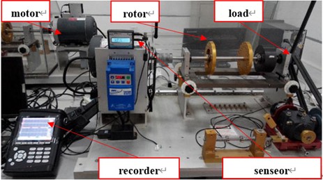
To revalidate the effectiveness of GSABO in rolling bearing diagnosis, verification tests were conducted using the XJTU-SY dataset [43]. The signal acquisition setup is illustrated on Fig. 13. Experiments were performed on a mechanical fault simulator (Spectra Quest Inc.) with seeded faults on NSK 6203 bearings (inner/outer races). Under a constant 1-horsepower load, vibration signals were meticulously collected at three rotational speeds (19.05 Hz, 29.05 Hz, 39.05 Hz) and three fault severity levels (mild, moderate, severe). The test rig comprised three core components: induction motor, rotor assembly, and loading system. A piezoelectric accelerometer (sensitivity: 50 mV/g) acquired motor bearing signals, with data recorded at 25.6 kHz sampling frequency using a CoCo80 data logger.

In this experiment, bearing data with a rotational frequency of 39.05 Hz was utilized, encompassing seven distinct fault conditions: normal operation, mild inner race fault, moderate inner race fault, severe inner race fault, mild outer race fault, moderate outer race fault, and severe outer race fault. Each fault signal contains 2048 sample points, with 120 samples collected per fault category (90 for training, 30 for testing).

Fig. 13XJTU-SY bearing fault diagnosis test rig

4.2.2. Fault signal decomposition

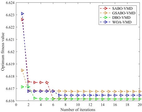
Taking the mild inner race fault as an example, the GSABO was configured with a population size of 15 and maximum iterations of 20 to optimize the decomposition level $k\in \left[\mathrm{3,10}\right]$ and penalty factor $\alpha \in \left[\mathrm{100,2500}\right]$. Using minimum envelope entropy as the objective function, the optimization yielded $\left(k,\alpha \right)=\left(\mathrm{4,164}\right)$. The optimization curve is shown on Fig. 14.

The GSABO achieved convergence in the 2nd generation, outperforming the baseline SABO (6th generation), DBO (4th generation), and WOA (7th generation). This experiment further demonstrates GSABO’s superior convergence characteristics.

The best parameter combinations and the best IMF components for each fault type are shown in Table 8.

Table 8Optimal VMD parameters and corresponding IMF components

Condition	Labels	$\left(k,\alpha \right)$	Optimal IMF
Normal	1	(10, 517)	IMF6
Minor internal ring fault	2	(5, 164)	IMF 3
Moderate internal ring fault	3	(3, 463)	IMF 3
Major internal ring fault	4	(4, 582)	IMF 2
Minor external ring fault	5	(8, 630)	IMF 7
Moderate external ring fault	6	(7, 319)	IMF 7
Major external ring fault	7	(4, 734)	IMF 4

Fig. 14Performance comparison of convergence curves

4.2.3. Fault feature identification

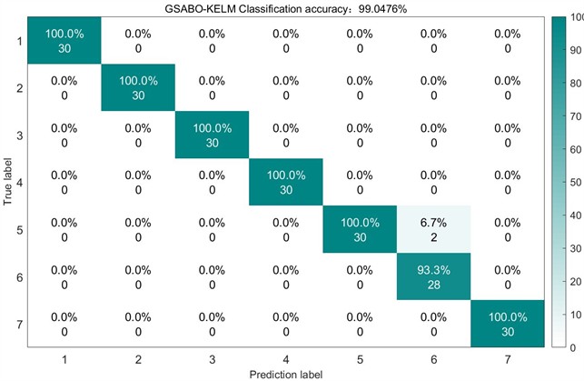
Consistent with the previous experiment, time-frequency domain features of the screened IMF components were computed as characteristic indicators to construct the fault feature vector matrix for GSABO-KELM classification. Using identical optimization parameters, the optimization process uses classification accuracy as the fitness function. The best parameter set $\left(C,g\right)=\left(\mathrm{402.775,0.205}\right)$ obtained through GSABO-KELM optimization yields an accuracy of 99.0476 %, while Fig. 15 displays the test set confusion matrix obtained through GSABO-VMD decomposition.

Fig. 15Confusion matrix of GSABO on the test set

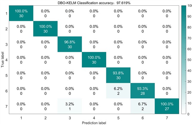
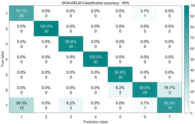
For control experiments, the unoptimized SABO, DBO, and WOA algorithms were employed for VMD decomposition of the sample data while maintaining identical feature extraction and classification procedures. The test set recognition accuracies achieved were 98.5417 % (SABO), 97.619 % (DBO), and 90 % (WOA) respectively. The corresponding test results and confusion matrices are presented in Figs. 16 through 18.

The confusion matrix analysis reveals that GSABO-VMD-KELM misclassified only two Label 6 fault samples as Label 1. Among the four optimization algorithms, GSABO-KELM achieved the fastest diagnostic speed at merely 6.31 seconds 2.35s faster than SABO-KELM (8.66s), 2.67s quicker than DBO-KELM (8.98s), and 4.11s swifter than WOA-KELM (10.42s). The improved SABO algorithm not only enhances diagnostic accuracy but also reduces processing time, demonstrating its superior performance in rolling bearing fault diagnosis.

Fig. 16Confusion matrix of SABO on the test set

Fig. 17Confusion matrix of DBO on the test set

5. Conclusions

In this paper, an optimized VMD based on GSABO decomposition of rolling bearing vibration signals is proposed. The IMF component obtained by the decomposition is screened by the envelope entropy, and then the time-frequency domain is calculated as the feature vector for feature extraction.

Fig. 18Confusion matrix of WOA on the test set

Finally, the GSABO optimized nuclear extreme learning machine is input to identify and diagnose the fault types. Through the analysis of experimental data, the following conclusions can be drawn:

1) The GSABO algorithm is employed to optimize the VMD parameters $k$ and $\alpha$, eliminating the need for manual or heuristic selection and effectively addressing the challenge of VMD parameter configuration.

2) To enhance the efficiency of the optimization algorithm and address the issue of getting trapped in local optima, a chaotic map and golden sine strategy were integrated to improve the SABO algorithm. Through testing the CEC2005 benchmark functions and comparisons of evolutionary curves, the GSABO algorithm demonstrates certain advantages over the original SABO and other optimization algorithms.

3) The GSABO-optimized KELM is employed to classify the feature vectors extracted from GSABO-VMD decomposition. By comparing the recognition results with those of unimproved SABO, DBO, and WOA optimized KELM and VMD, the advancement of the proposed method is demonstrated. Further validation is conducted using rolling bearing vibration signals from CWRU and XJTU, the accuracy rates reached 99.3333 % and 99.0476 %, respectively, confirming the effectiveness of the proposed method in rolling bearing fault identification. This approach provides valuable insights for research in the field of rolling bearing fault diagnosis.

Although the proposed method demonstrates satisfactory performance in rolling bearing fault diagnosis, certain limitations need to be addressed. The present research is confined to vibration signal analysis, whereas industrial practice involves additional measurable parameters (e.g., temperature, current) that contain critical equipment, health information. Subsequent studies will focus on developing multi-sensor data fusion techniques to deliver more reliable and informative diagnostic solutions for maintenance engineers.